Estimate Net AEP and P90 AEP

Example of estimating the Net AEP and P90 AEP using a loss table and an uncertainty table. For a more detailed overview see PyWAsP Tutorial 6.

First, we calculate the Gross AEP and the Potential AEP of the wind farm in the Serra Santa Luzia tutorial data.

import pywasp as pw
import windkit as wk
import numpy as np
import matplotlib.pyplot as plt
from scipy.stats import norm

ssl = wk.load_tutorial_data("serra_santa_luzia")
# The wind directions are relative to the grid north of the UTM 29N maps
bwc = ssl.bwc.assign_attrs(wind_dir_crs="EPSG:32629")
topo_map = pw.wasp.TopographyMap(ssl.elev, ssl.rgh)
wwc = pw.wasp.predict_wwc(bwc, topo_map, ssl.turbines)

gross_aep = pw.gross_aep(wwc, ssl.wtg)
potential_aep = pw.potential_aep(wwc, ssl.wtg)

Losses towards P50 - Importing a loss table

loss_table = wk.get_loss_table("dtu_default")

# Modify loss values as needed
loss_table.loc[0, "loss_percentage"] = 0.5
loss_table.loc[2, "loss_percentage"] = 0.1

print(loss_table.head())

                    loss_name  ...                                        description
0        turbine_availability  ...  Turbine availability losses, including downtim...
1  balance_plant_availability  ...  Balance of plant availability losses, includin...
2           grid_availability  ...  Grid availability losses, excluding curtailmen...
3        electrical_operation  ...  Electrical losses, including transformer and c...
4              wf_consumption  ...  Wind farm consumption losses, including auxili...

[5 rows x 7 columns]

Losses towards P50 - Calculating the Net AEP

net_aep = pw.net_aep(loss_table, potential_aep)
print("Net AEP:", net_aep["net_aep"].values.sum(), "GWh")

Net AEP: 39.347850665091514 GWh

Uncertainties towards P90 - Importing a uncertainty table

uncertainty_table = wk.get_uncertainty_table()
print(uncertainty_table.head())
print(uncertainty_table.tail())

  uncertainty_kind  ...                                        description
0             wind  ...  Uncertainty associated with the statistical re...
1             wind  ...  Uncertainty associated with the accuracy or re...
2             wind  ...  Uncertainty associated with the MCP process, i...
3             wind  ...  Uncertainty associated with the representative...
4             wind  ...  Uncertainty associated with gap-filling missin...

[5 rows x 8 columns]
   uncertainty_kind  ...                                        description
29           energy  ...  Uncertainty associated with exposure changes l...
30           energy  ...  Uncertainty associated with load curtailment l...
31           energy  ...  Uncertainty associated with grid curtailment l...
32           energy  ...  Uncertainty associated with environmental curt...
33           energy  ...  Uncertainty associated with operational strate...

[5 rows x 8 columns]

Note

Terms that are part of the “energy” kind are those related to the uncertainties of the technical losses. Terms that are part of the “wind” kind are those related to the uncertainties of the predicted wind climate.

Uncertainties towards P90 - Calculating the Px yield

Note

For a P90 value, x = 90.

p90 = pw.px_aep(uncertainty_table, net_aep, sensitivity_factor=1.5, percentile=90)
print("The P90 is:", p90["P_90_aep"].values.sum(), "Gwh")

The P90 is: 34.95598991055112 Gwh

tot_sigma, _, _ = wk.total_uncertainty(uncertainty_table, 1.5)
p50 = np.round(net_aep["net_aep"].values.sum(), 2)
sigma_tot_dimensional = np.round(tot_sigma / 100 * p50, 2)

plt.figure(figsize=(14, 6))

x = np.linspace(15, 60, 100)

plt.axvline(
    gross_aep["gross_aep"].values.sum(),
    color="k",
    linestyle="-.",
    linewidth=2,
    label="Gross AEP mean",
)
plt.axvline(
    potential_aep["potential_aep"].values.sum(),
    color="b",
    linestyle="--",
    alpha=0.7,
    linewidth=2,
    label="Potential AEP mean",
)
plt.axvline(p50, color="r", linestyle="solid", linewidth=2, label="P50")
plt.axvline(
    p50 + sigma_tot_dimensional,
    color="r",
    linestyle="dashed",
    linewidth=1,
    label="P50 -+ σ",
)
plt.axvline(p50 - sigma_tot_dimensional, color="r", linestyle="dashed", linewidth=1)
plt.axvline(
    p90["P_90_aep"].values.sum(), color="g", linestyle="-.", linewidth=1.5, label="P90"
)
pdf = norm.pdf(x, p50, sigma_tot_dimensional)
plt.plot(x, pdf, color="r", linewidth=2, alpha=0.5)

plt.grid(True)
plt.legend()
plt.title("Gaussian distributio of the AEP")
plt.xlabel("AEP [GWh]")

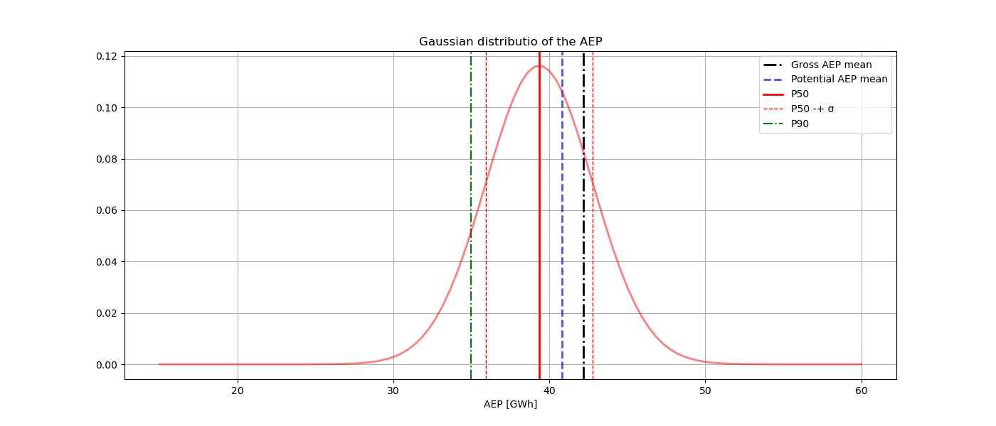
Text(0.5, 36.72222222222221, 'AEP [GWh]')