Fitting Weibull Distributions

This example demonstrates how to fit Weibull parameters to a wind speed distribution using the moments-based Weibull fitting method used by WAsP.

Lets start by fiting Weibull parameters to a known first moment (the mean wind speed), third moment, and the frequency fraction that is greater than the mean (first moment). To fit the Weibull parameters, we will use the windkit.weibull.fit_weibull_wasp_m1_m3_fgtm() function.

import windkit as wk
import numpy as np
from scipy.stats import weibull_min
import matplotlib.pyplot as plt

first_moment = 7.0
third_moment = 600.0
freq_gt_mean = 0.46

A, k = wk.weibull.fit_weibull_wasp_m1_m3_fgtm(first_moment, third_moment, freq_gt_mean)
print(f"Weibull A: {A:.2f}, k: {k:.2f}")

Weibull A: 7.87, k: 2.16

Deriving relevant statistics from a wind speed distribution

Now, let’s go back and instead start from a wind speed distribution and derive the first moment, third moment, and frequency fraction greater than the mean. We will use a Weibull distribution with the known parameters from above.

size = 100_000  # number of samples
ws_samples = weibull_min.rvs(k, loc=0, scale=A, size=size, random_state=0)

bins = np.linspace(0.0, 30.0, 31)
centers = 0.5 * (bins[:-1] + bins[1:])
ceils = np.ceil(centers)

hist, bin_edges = np.histogram(ws_samples, bins=bins, density=True)

Caculate statistics

Now, we can calculate the first moment, third moment, and the frequency fraction greater than the mean

first_moment = centers @ hist
third_moment = (centers**3) @ hist
cdf = np.cumsum(hist)
freq_gt_mean = 1.0 - np.interp(first_moment, ceils, cdf)


print(f"First Moment: {first_moment:.2f} m/s")
print(f"Third Moment: {third_moment:.2f} m^3/s^3")
print(f"Frequency Fraction Greater Than Mean: {freq_gt_mean:.2f}")

First Moment: 6.96 m/s
Third Moment: 602.24 m^3/s^3
Frequency Fraction Greater Than Mean: 0.46

Fit Weibull distribution using the calculated moments

A_fit, k_fit = wk.weibull.fit_weibull_wasp_m1_m3_fgtm(
    first_moment, third_moment, freq_gt_mean
)
print(f"Fitted Weibull A: {A_fit:.2f}, k: {k_fit:.2f}")

Fitted Weibull A: 7.87, k: 2.16

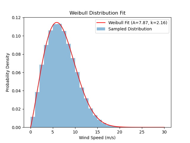
Visualizing the distribution

x = np.linspace(0, 30, 1000)

plt.bar(
    centers,
    hist,
    width=np.diff(bins),
    align="center",
    alpha=0.5,
    label="Sampled Distribution",
)
plt.plot(
    x,
    weibull_min.pdf(x, k_fit, loc=0, scale=A_fit),
    label=f"Weibull Fit (A={A_fit:.2f}, k={k_fit:.2f})",
    color="red",
)
plt.legend()
plt.xlabel("Wind Speed (m/s)")
plt.ylabel("Probability Density")
plt.title("Weibull Distribution Fit")

Text(0.5, 1.0, 'Weibull Distribution Fit')