[1]:
%load_ext autoreload
%autoreload 2
[2]:
import os
import warnings
warnings.filterwarnings('ignore') # We will ignore warnings to avoid cluttering the notebook
import numpy as np
import matplotlib.pyplot as plt
import windkit as wk
import pywasp as pw
from tutorial_helpers import (
read_tabfiles_oesterild,
set_config,
plot_transect_ws,
plot_transect_pd,
plot_profile,
plot_transect_z0,
plot_transect_displ,
)
Evaluating roughness maps at Østerild#
In this tutorial you will use several new features related to the treatment of roughness maps; these functionalities are not available in the WAsP GUI, but have been developed using the pywasp interface. Data from the Danish national test center for large wind turbines at Østerild will be used: there are two meteorological masts located to the north and south of a row of turbines (red and black points in figure below, respectively). The masts have measurements up to 244 m height, and are
instrumented with both cup and sonic anemometers. The wind data used in this exercise are quality-controlled: periods where wakes and icing influenced the measurements have been removed. In addition, sectors that were influenced by the wakes of nearby turbines have been filtered out: this causes some sectors to have no observations (tripping a warning when reading the observed wind climates).
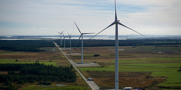
Picture source: innowind.dk
Østerild wind data from Dec. 13th of 2016 to May 24th of 2018 (71802 10-min measurements) are used, with the following data and processing details:
data available from both northern and southern masts (red triangles in figure below);
icing episodes removed by selecting data with standard deviation
 m/s;
m/s;flow distortion correction via “Flow distortion on boom-mounted cup anemometers” (P. Lindelöw-Marsden et al.);
wind directions linearly interpolated between 40 and 244 m;
data from sectors with wind turbine wakes were removed;
12-sector histogram files were already generated using
pywasp.
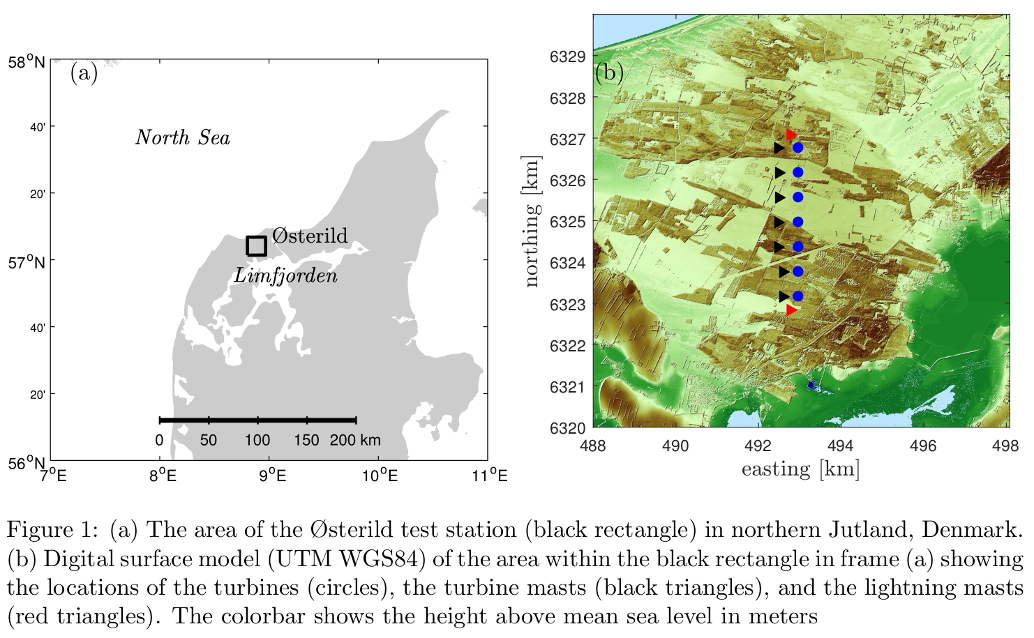
Above figure source: Peña et al. (2019)
Reading Østerild wind data#
First we will read mast data from the two masts; these have been stored as multiple tab files, and are read using the “helper” function read_tabfiles_oesterild made for this tutorial.
[3]:
tabs = read_tabfiles_oesterild()
print(tabs)
<xarray.Dataset> Size: 63kB
Dimensions: (sector: 12, point: 16, wsbin: 39)
Coordinates:
height (point) float64 128B 10.0 40.0 70.0 ... 178.0 210.0 244.0
crs int8 1B 0
wsceil (wsbin) float64 312B 1.0 2.0 3.0 4.0 ... 36.0 37.0 38.0 39.0
wsfloor (wsbin) float64 312B 0.0 1.0 2.0 3.0 ... 35.0 36.0 37.0 38.0
sector_ceil (sector) float64 96B 15.0 45.0 75.0 ... 285.0 315.0 345.0
sector_floor (sector) float64 96B 345.0 15.0 45.0 ... 255.0 285.0 315.0
* wsbin (wsbin) float64 312B 0.5 1.5 2.5 3.5 ... 35.5 36.5 37.5 38.5
* sector (sector) float64 96B 0.0 30.0 60.0 90.0 ... 270.0 300.0 330.0
west_east (point) float64 128B 4.928e+05 4.928e+05 ... 4.928e+05
south_north (point) float64 128B 6.323e+06 6.323e+06 ... 6.327e+06
Dimensions without coordinates: point
Data variables:
wdfreq (sector, point) float64 2kB 0.0 0.0 0.0 ... 0.04364 0.04703
wsfreq (wsbin, sector, point) float64 60kB 0.0 0.0 0.0 ... 0.0 0.0
Attributes:
Conventions: CF-1.8
history: 2025-03-28T14:11:06+00:00:\twindkit==0.8.2.dev20+g699a5...
description: Mast 2 10 m from timeseries
Package name: windkit
Package version: 0.8.2.dev20+g699a596.d20250328
Creation date: 2025-03-28T14:11:06+00:00
Object type: Binned Wind Climate
author: Bjarke Tobias OLsen
author_email: btol@dtu.dk
institution: DTU Wind Energy
header: Binned wind climates (bwc) from Østerild from the North...
We note in the Dimensions of the xarray.Dataset that was read as tabs shows 16 points; the first 8 points correspond to the South mast, while the last 8 points correspond to the Northern mast.
These are binned wind climate files, whose format was explained earlier in the resource grid tutorial. I.e., there are no mean speeds, but rather probabilities (frequencies of occurence) per wind speed bin (wsbin) and directional sector stored in wsfreq (with directional probabilities over all speeds in wdfreq).
Preparing map files#
Traditionally WAsP has only been able to use vector maps for roughness length. In pywasp it is very easy to work with both raster (grid) and vector (contour) maps, with simple functions to convert between formats.
In this tutorial we’ll load raster map files from a number of sources, in the following order:
Danish Digital Terrain-elevation Map (DTM). For the description of the terrain height we use the digital elevation model from Denmark’s Geodatastyrelsen, at a resolution of 100 m (the full dataset was obtained via airplane-based lidar scans, and much finer resolutions can also be downloaded).
CORINE landcover. The European Union’s CORINE initiative (‘COoRdination of INformation on the Environment’) is popular for wind resource assessments in Europe, due to its relatively fine resolution of 100 m (e.g. it is used for land cover in the New European Wind Atlas).
Sentinel satellite data. Through the INNOWIND project, which aims to use new information from satellites to create more accurate wind resource assessments, a new land cover product has been created. It has 20 m resolution and provides not just landcover classes, but also tree height and leaf area index in forested areas.
[4]:
elev_ras = wk.read_elevation_map(
os.path.join('data/maps','Oesterild_DTM_100m.grd'),
crs=32632
)
After reading the raster map of terrain elevation above, we now convert it to a vector map using the pywasp.io.raster_to_vector function previously outlined and used in the tutorial on resource grids.
[5]:
elev_map = pw.raster_to_vector(elev_ras)
To load a raster map where each grid-cell (pixel) represents a roughness length, we can specify that we are loading a map of type 'roughness' within the read_rastermap function.
pywasp note: it is a neccessary step for roughness data in raster format to be converted to vector representation , because
pywaspcan only work with vector maps.
[6]:
corine_z0_ras= wk.read_roughness_map(
os.path.join('data/maps','corine.grd'),
crs=32632
)
corine_z0_map = pw.raster_to_vector(corine_z0_ras)
Using landcover (LC) maps#
Above we loaded raster mapfiles with commonly-used elevation and roughness length data, and transformed them to vector format; along with reading the roughness lengths we converted them to landcover classes, also getting a corresponding lookup table.
But what if we have LC maps, and not  ? This is actually the case for the Sentinel data.
Below we see how to load a raster map of landcover and corresponding landcover tables, using the pw.LandCoverTable.read_json and pw.read_rastermap methods (the cells in the map represent landcover classes, which correspond to the in the lookup table).
This is done for both the CORINE data and the Sentinel data, along with converting each map to vector format:
[7]:
corine_lctable = pw.LandCoverTable.read_json(os.path.join('data/maps','corine_DTU.json'))
corine_ras = wk.read_landcover_map(os.path.join('data/maps','corine_lu.grd'), crs=32632)
corine_map = pw.raster_to_vector(corine_ras)
sentinel_lctable = pw.LandCoverTable.read_json(os.path.join('data/maps','scadis_sentinel.json'))
sentinel_ras = wk.read_landcover_map(os.path.join('data/maps','sentinel.tif'), crs=32632)
sentinel_map = pw.raster_to_vector(sentinel_ras)
Roughness and landcover around masts#
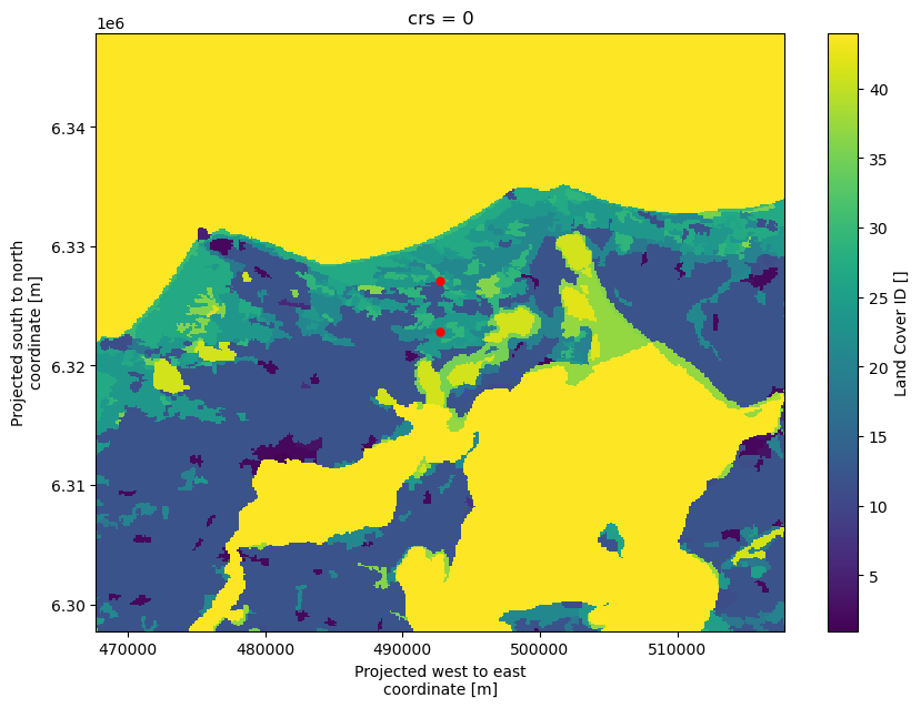
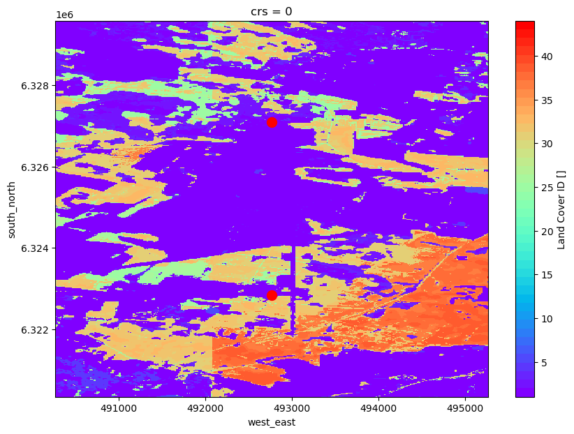
Let’s explore the maps that have been loaded, using the ‘plot()’ method of xarray (recalling that 'corine_ras' is an xarray DataArray, and find the approximate roughness and landcover classes around the masts. We also use red dots to show the locations of the masts, which were contained in the 'tabs' variable created by reading the wind data at the beginning of this tutorial.
[8]:
x_mastS = tabs['west_east'][0]
x_mastN = tabs['west_east'][15]
y_mastS = tabs['south_north'][0]
y_mastN = tabs['south_north'][15]
[9]:
corine_ras.plot(figsize=(10,7))
plt.plot(x_mastN, y_mastN, 'or', ms=5)
plt.plot(x_mastS, y_mastS, 'or', ms=5)
plt.show()
we can zoom in more (limiting the plot area using xlim and ylim) and make the color bar discrete (noting there are 44 LC types in 'corine_ras' and changing the color-map), to better see the LC’s around the masts:
[10]:
rzoom = 2500
my_cmap=plt.get_cmap('terrain', 44)
corine_ras.plot(figsize=(10,7), cmap=my_cmap)
plt.plot(x_mastN, y_mastN, 'or', ms=5)
plt.plot(x_mastS, y_mastS, 'or', ms=5)
plt.xlim([x_mastS - rzoom, x_mastS + rzoom])
plt.ylim([y_mastS - rzoom, y_mastN + rzoom])
plt.show()
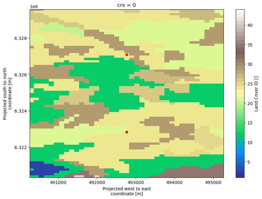
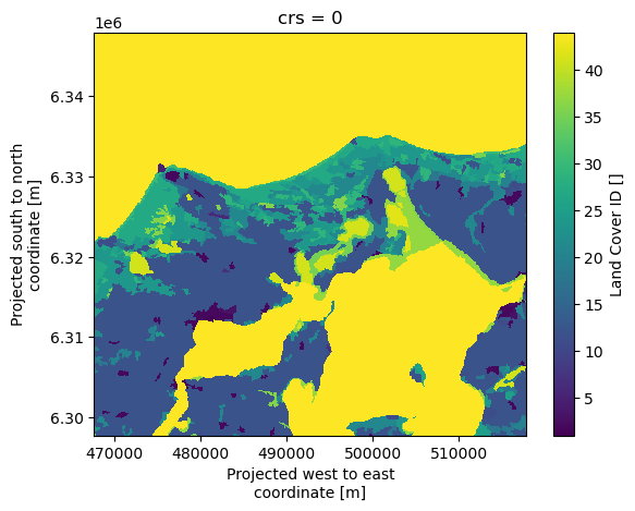
From the CORINE map we can find out that much of the LandCoverID around the mast locations is 24, which according to the CORINE look-up table corresponds to “Coniferous forest” or z0 = 1.2. On the other hand, from the Sentinel map LandCoverID for the mast locations is 1, which corresponds to “non-forest (cropland grassland other)” or z0 = 0.1.
[11]:
sentinel_ras.plot(figsize=(10,7), cmap=plt.get_cmap('rainbow', 44))
plt.plot(x_mastN, y_mastN, 'or', ms=10)
plt.plot(x_mastS, y_mastS, 'or', ms=10)
plt.xlim([x_mastS - rzoom, x_mastS + rzoom])
plt.ylim([y_mastS - rzoom, y_mastN + rzoom])
plt.show()
As seen above, the Sentinel data in this case appears to include much more detail than CORINE; e.g. we can see line-like features where the forests have been cut. (Note: water is class 5 in the Sentinel lookup-table, where the classes are not ordered according to . We have picked a different color table to accomodate this and make it blue. You can check the LC() by simply looking at sentinel_lctable.)
Now we combine the vector elevation map obtained earlier with the CORINE and Sentinel landcover vector maps and CORINE z0 vector map, and make a TopographyMap for each pair. Such combination of elevation and roughness/landcover maps is done, because they are both needed for the flow modelling in WAsP/pywasp. Here we store them in a dictionary ('allmaps') for further processing:
[12]:
allmaps = {}
allmaps['Sentinel landcover'] = pw.wasp.TopographyMap(elev_map, sentinel_map, sentinel_lctable)
allmaps['CORINE landcover']= pw.wasp.TopographyMap(elev_map, corine_map, corine_lctable)
allmaps['CORINE z0']= pw.wasp.TopographyMap(elev_map, corine_z0_map)
[13]:
corine_ras.plot()
plt.show()
Exploring roughness around a point: the roughness rose#
WAsP’s internal boundary layer (IBL) model computes speedup effects due to (a limited number of) the most significant roughness changes in each directional sector; this was discussed in the earlier tutorial on (py)WAsP’s response to roughness changes. A roughness rose can be plotted, which displays the sector-wise as a function of distance.
But to use WAsP’s roughness-change model, and for displaying -roses, we must set up pywasp’s configuration. This was also briefly covered/used in the resource_grid tutorial.
Here we use the default WAsP configuration, but additionally employ the new landcover roughness model; the latter adds the ability to deal with displacement heights, i.e. treating flow that is “displaced” upward over forests based on mean tree height and leaf-area density (as found e.g. via Sentinel data).
pywasp note: WAsP has about 60 parameters and constants that can be changed to control the behaviour of its various submodels, most importly those involving terrain-induced perturbations, vertical extrapolation, and getting/applying generalized wind statistics.
To get an overview of the settings of the various parameters, you can print the conf.terrain and conf.climate configurations. In practice we occasionally adjust only a small fraction of parameters from their default values, just as in WAsP, though further research and use of pywasp may change this; also, only some are actually visible to end-users. In-depth docummentation of them (beyond the European Wind Atlas, 1989) is currently under way, though one can use getpardesc(pno) for
parameter number pno to get some description (done below).
[14]:
conf = set_config()
conf.terrain
[14]:
Index Parameter Current Default Description
value value
===== ========================== ============ =========== ==================================================
31 decay_length 10000.000000 10000 Decay-length for importance of roughness relative to distance from center
40 upper_kink_ibl_profile 0.300000 0.3 Factor for upper kink in roughness change wind profile in the ibl
41 lower_kink_ibl_profile 0.090000 0.09 Factor for lower kink in roughness change wind profile in the ibl
67 max_no_roughness_changes 10.000000 10 Max number of roughness changes/sector. See \cite{Floors2018b} for description and sensitivity. This array is dimensioned in the variable mrchs in dimpar.f90.
68 max_rms_error 0.300000 0.3 Maximum root-mean square (rms) error in log(roughness) analysis of roughness changes for a given sector. Setting a lower error threshold will allow a higher number of roughness changes to be taken into consideration, for each sector. Choosing 0 causes this parameter to become inactive, with the maximum number of changes then set by parameter~67.
69 use_displacement_height 1.000000 1 add displacements to orographic grid if = 1, and reduce displacement slope near origin to parameter~70
82 roughness_analysis 1.000000 1 rou analysis version: 0=old, =1 use spiderweb with old rou maps
97 water_roughness_length 0.000200 0.0002 ($2\times10^{-4}$) water roughness length used in program
[15]:
conf.terrain.get_desc(67)
================================================================================
max_no_roughness_changes
================================================================================
standard_name : max_no_of_roughness_changes
short_name : max_no_roughness_changes
long_name : max_no_of_roughness_changes_per_sector
GUID : MAXRC
Rvea : Rvea0287
model : IBL/roughness-change model
index : 67
valid_min : 1
valid_max : 20
valid_range : [1, 20]
default_value : 10
definition:
Max number of roughness changes/sector. See \\cite{Floors2018b} for
description and sensitivity. This array is dimensioned in the variable mrchs
in dimpar.f90.
================================================================================
[16]:
conf.terrain.get_desc(31)
================================================================================
decay_length
================================================================================
standard_name : roughness_decay_length
short_name : decay_length
long_name : Decay-length for roughness area size
GUID : RDECAYL
Rvea : Rvea0287
model : WAsP IBZ flow modelling
index : 31
units : m
valid_min : 1000
valid_max : 1000000
valid_range : [1000, 1000000]
default_value : 10000
definition:
Decay-length for importance of roughness relative to distance from center
reference : European Wind Atlas---\cite{Troen1989}, around equation~8.24
notes:
("Used to get 'meso'-roughness: determines relative weight to roughnesses "
'depending on distance from wind calculation point (center).
================================================================================
To see the roughness roses of all maps at a certain location we can do the following:
loop over all maps stored in the dictionary
'allmaps'use the
selmethod from xarray to select the first point intabs(South mast, height = 10 m viapoint=0)[also possible: select the site factors using the ``to_point`` method]
plot a roughness rose for each map
NOTE: we arbitrarily select from 10 m height, because the roughness rose does not depend on height
[17]:
tabs0 = tabs.sel(point=0)
south_mast_loc = wk.spatial.create_dataset(
tabs0.west_east,
tabs0.south_north,
tabs0.height,
wk.spatial.get_crs(tabs0)
)
for key, topo_map in allmaps.items():
print(key)
rou_rose, _ = topo_map.get_rou_rose(south_mast_loc, n_sectors=12, conf=conf)
wk.plot.roughness_rose(rou_rose)
Sentinel landcover
CORINE landcover
CORINE z0
Comparison of observed and modelled wind, per roughness maps#
We can now proceed with a comparison between the observed and modelled wind speed (and its distribution), using the WAsP model to vertically extrapolate the measurements from a certain height to another; the wind profile and thus this extrapolation depends upon .
To start we first need to generalize the observed wind climate, after “cleaning” local terrain effects from the wind observations; then after downscaling the generalized wind climate, we re-apply local effects for another height or location. The processes are performed by the generalize and downscale methods, as shown in the earlier tutorial on resource maps.
Below we select observations from a certain height and mast and create a generalized wind climate (gwc) from them:
the first argument is input binned wind climate (remember first 8 points correspond to the South mast, remaining to the North mast)
the second argument is the mapfile that we want to use to generalize the observations
the third argument is the WAsP model configuration
[18]:
bwc = tabs.sel(point=3, drop=False) # Selecting wind data from the south mast at 106 m above ground level
gwc = pw.wasp.generalize(
bwc,
allmaps['Sentinel landcover'],
conf
)
[19]:
print(gwc)
<xarray.Dataset> Size: 4kB
Dimensions: (point: 1, sector: 12, gen_height: 5, gen_roughness: 5)
Coordinates:
height (point) float64 8B 106.0
south_north (point) float64 8B 6.323e+06
west_east (point) float64 8B 4.928e+05
crs int8 1B 0
sector_ceil (sector) float64 96B 15.0 45.0 75.0 ... 285.0 315.0 345.0
sector_floor (sector) float64 96B 345.0 15.0 45.0 ... 255.0 285.0 315.0
* sector (sector) float64 96B 0.0 30.0 60.0 90.0 ... 270.0 300.0 330.0
* gen_roughness (gen_roughness) float64 40B 0.0 0.03 0.1 0.4 1.5
* gen_height (gen_height) int64 40B 10 25 50 100 250
Dimensions without coordinates: point
Data variables:
A (sector, gen_height, gen_roughness, point) float32 1kB 6.8...
k (sector, gen_height, gen_roughness, point) float32 1kB 1.9...
wdfreq (sector, gen_height, gen_roughness, point) float32 1kB 0.0...
site_elev (point) float32 4B 10.15
Attributes:
Conventions: CF-1.8
history: 2025-03-28T14:11:06+00:00:\twindkit==0.8.2.dev20+g699a5...
description: Mast 2 10 m from timeseries
Package name: windkit
Package version: 0.8.2.dev20+g699a596.d20250328
Creation date: 2025-03-28T14:12:30+00:00
Object type: Geostrophic Wind Climate
author: Bjarke Tobias OLsen
author_email: btol@dtu.dk
institution: DTU Wind Energy
header: Binned wind climates (bwc) from Østerild from the North...
title: Generalized wind climate
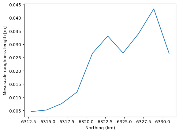
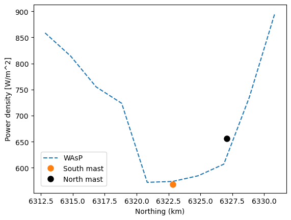
Horizontal transects of power density#
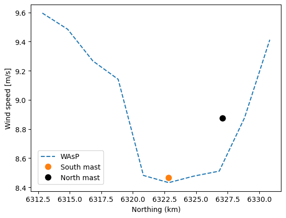
Now that we have a generalized wind climate, we can reapply this wind climate for any nearby location. In this case we will create a horizontal transect of locations along a line connecting the meteorological masts, from 10 km south to 10 km north, at 106 m above ground level. The coordinates of the mast are taken from bwc. The output of the downscale function is a Weibull wind climate ('wwc'), i.e. sector-wise Weibull distributions at our transect.
[20]:
loc_x = float(bwc.west_east)
loc_y = float(bwc.south_north)
half_ext = 10000.0 # half extent in x and y in m
points_y = np.arange(loc_y-10000,loc_y+10000,2000)
transect = wk.spatial.create_point(
west_east=np.repeat(loc_x,len(points_y)),
south_north=points_y,
height=np.repeat(bwc.height.values,len(points_y)),
crs=32632
)
wwc = pw.wasp.downscale(
gwc,
allmaps['Sentinel landcover'],
transect,
conf,
interp_method='nearest'
)
[21]:
plot_transect_z0(tabs,transect,allmaps['CORINE landcover'],conf)
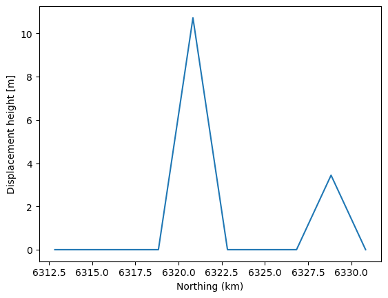
[22]:
plot_transect_displ(tabs,transect,allmaps['Sentinel landcover'],conf)
[23]:
plot_transect_ws(tabs,wwc)
[24]:
plot_transect_pd(tabs,wwc)
Vertical profile of power density#
Instead of a horizontal transect, we can also easily plot a vertical profile of the power density. For this a we can use the function wk.plot_vertical_profile. It takes the same arguments as the plot_transect_pd function, i.e. the dataset of binned wind climates and a Weibull wind climate. To do this we will:
Use the
create_gridfunction to create the output locations for the flow modellingPerform the downscaling step as described in the section “Validation of roughness maps”. We can use the same generalized wind climate as before.
Call the
wk.plot_vertical_profilefunction using the objects that have been created in the previous two steps
Let’s do this first for the South mast:
[25]:
print(tabs)
<xarray.Dataset> Size: 63kB
Dimensions: (sector: 12, point: 16, wsbin: 39)
Coordinates:
height (point) float64 128B 10.0 40.0 70.0 ... 178.0 210.0 244.0
crs int8 1B 0
wsceil (wsbin) float64 312B 1.0 2.0 3.0 4.0 ... 36.0 37.0 38.0 39.0
wsfloor (wsbin) float64 312B 0.0 1.0 2.0 3.0 ... 35.0 36.0 37.0 38.0
sector_ceil (sector) float64 96B 15.0 45.0 75.0 ... 285.0 315.0 345.0
sector_floor (sector) float64 96B 345.0 15.0 45.0 ... 255.0 285.0 315.0
west_east (point) float64 128B 4.928e+05 4.928e+05 ... 4.928e+05
south_north (point) float64 128B 6.323e+06 6.323e+06 ... 6.327e+06
* wsbin (wsbin) float64 312B 0.5 1.5 2.5 3.5 ... 35.5 36.5 37.5 38.5
* sector (sector) float64 96B 0.0 30.0 60.0 90.0 ... 270.0 300.0 330.0
Dimensions without coordinates: point
Data variables:
wdfreq (sector, point) float64 2kB 0.0 0.0 0.0 ... 0.04364 0.04703
wsfreq (wsbin, sector, point) float64 60kB 0.0 0.0 0.0 ... 0.0 0.0
air_density (point) float64 128B 1.225 1.225 1.225 ... 1.225 1.225 1.225
wspd (point) float64 128B 4.159 6.075 7.363 ... 10.22 10.62 10.93
power_density (point) float64 128B 99.46 240.3 ... 1.148e+03 1.263e+03
Attributes:
Conventions: CF-1.8
history: 2025-03-28T14:11:06+00:00:\twindkit==0.8.2.dev20+g699a5...
description: Mast 2 10 m from timeseries
Package name: windkit
Package version: 0.8.2.dev20+g699a596.d20250328
Creation date: 2025-03-28T14:12:33+00:00
Object type: Met fields
author: Bjarke Tobias OLsen
author_email: btol@dtu.dk
institution: DTU Wind Energy
header: Binned wind climates (bwc) from Østerild from the North...
[26]:
loc_x = tabs.west_east.values[0] # selecting the South mast x coordinate
loc_y = tabs.south_north.values[0] # selecting the South mast y coordinate
heights = tabs.height.values[:8] # selecting the South mast heights
bwc_smast= tabs.isel(point=range(0,8)) # South mast data
transect = wk.spatial.create_point(
west_east=np.repeat(loc_x,len(heights)),
south_north=np.repeat(loc_y,len(heights)),
height=heights,
crs=32632
)
wwc_south = pw.wasp.downscale(
gwc,
allmaps['Sentinel landcover'],
transect,
conf,
interp_method='nearest'
)
[27]:
wk.plot.vertical_profile(bwc_smast.power_density,wwc_south.power_density)
We will repeat the previous calculations for the North mast:
[28]:
loc_xN = tabs.west_east.values[8] # selecting the North mast x coordinate
loc_yN = tabs.south_north.values[8] # selecting the North mast y coordinate
heightsN = tabs.height.values[8:] # selecting the North mast heights
bwc_nmast= tabs.isel(point=range(8,16)) # North mast data
transect = wk.spatial.create_point(
west_east=np.repeat(loc_xN,len(heights)),
south_north=np.repeat(loc_yN,len(heights)),
height=heightsN,
crs=32632
)
wwc_north = pw.wasp.downscale(
gwc,
allmaps['Sentinel landcover'],
transect,
conf,
interp_method='nearest'
)
wk.plot.vertical_profile(bwc_nmast.power_density,wwc_north.power_density)
Changing properties of the landcover data#
The advantage of using a landcover file together with a landcover table is that it easy to change the properties of the landcover. Let’s start by showing the content of the CORINE landcover table that we loaded before:
[29]:
print(corine_lctable)
id = LandCoverID
z0 = Roughness length (m)
d = Displacement height (m)
desc = Description
id z0 d desc
0 0.0000 0.0 no datanull
48 0.0000 0.0 no datanull
255 0.0000 0.0 no datanull
1 1.0000 0.0 Continuous urban fabric 111
2 0.8000 0.0 Discontinuous urban fabric 112
3 0.7000 0.0 Industrial or commercial units 121
4 0.1000 0.0 Road and rail networks and associated land 122
5 0.5000 0.0 Port areas 123
6 0.0100 0.0 Airports 124
7 0.0500 0.0 Mineral extraction sites 131
8 0.0500 0.0 Dump sites 132
9 0.3000 0.0 Construction sites 133
10 0.8000 0.0 Green urban areas 141
11 0.2000 0.0 Sport and leisure facilities 142
12 0.0500 0.0 Non-irrigated arable land 211
13 0.0300 0.0 Permanently irrigated land 212
14 0.0300 0.0 Rice fields 213
15 0.3000 0.0 Vineyards 221
16 0.4000 0.0 Fruit trees and berry plantations 222
17 0.4000 0.0 Olive groves 223
18 0.0300 0.0 Pastures 231
19 0.1000 0.0 Annual crops associated with permanent crops 241
20 0.1500 0.0 Complex cultivation patterns 242
21 0.2000 0.0 Land principally occupied by agriculture with significant areas of natural vegetation 243
22 0.5000 0.0 Agro-forestry areas 244
23 1.0000 0.0 Broad-leaved forest 311
24 1.2000 0.0 Coniferous forest 312
25 1.1000 0.0 Mixed forest 313
26 0.0300 0.0 Natural grasslands 321
27 0.0500 0.0 Moors and heathland 322
28 0.0700 0.0 Sclerophyllous vegetation 323
29 0.4000 0.0 Transitional woodland-shrub 324
30 0.0030 0.0 Beaches - dunes - sands 331
31 0.0500 0.0 Bare rocks 332
32 0.0300 0.0 Sparsely vegetated areas 333
33 0.2000 0.0 Burnt areas 334
34 0.0050 0.0 Glaciers and perpetual snow 335
35 0.0500 0.0 Inland marshes 411
36 0.0300 0.0 Peat bogs 412
37 0.0200 0.0 Salt marshes 421
38 0.0050 0.0 Salines 422
39 0.0000 0.0 Intertidal flats 423
40 0.0000 0.0 Water courses 511
41 0.0000 0.0 Water bodies 512
42 0.0000 0.0 Coastal lagoons 521
43 0.0000 0.0 Estuaries 522
44 0.0000 0.0 Sea and ocean 523
In the section ‘Roughness and landcover around masts’ we have seen that the land around the masts is dominated by category 24: coniferous forest, which according to the lookup table corresponds to  m. The assignment of the roughness length of forest comes with considerable uncertainty. We can make the assignment of roughness more objective by taking into account more parameters of the forest. The SCADIS 1d model available in WAsP can more accurately model the roughness length and
displacement height of a forest, using the following additional parameters:
m. The assignment of the roughness length of forest comes with considerable uncertainty. We can make the assignment of roughness more objective by taking into account more parameters of the forest. The SCADIS 1d model available in WAsP can more accurately model the roughness length and
displacement height of a forest, using the following additional parameters:
z0s: background roughness length, in metersh: mean tree height, in meterslai: leaf area indexalpha: shape parameter of leaf area density profilebeta: shape parameter of leaf area density profile
Below we assign some ad-hoc but plausible parameters for the forest around the two masts, i.e. a mean tree height of 20m and a leaf-area index of 3. Afterwards we run the SCADIS 1d model to convert these values to a roughness length. We print the landcover table to confirm that landcover index 24 has now a modified roughness length and displacement height.
[30]:
corine_lctable[24]={'z0s':0.3,'h':20,'lai':3,'alpha':3,'beta':3,'desc':'SCADIS 1D'}
corine_lctable.from_dict_scadis(corine_lctable)
[30]:
{0: {'z0': 0.0, 'd': 0.0, 'desc': 'no datanull'},
48: {'z0': 0.0, 'd': 0.0, 'desc': 'no datanull'},
255: {'z0': 0.0, 'd': 0.0, 'desc': 'no datanull'},
1: {'z0': 1.0, 'd': 0.0, 'desc': 'Continuous urban fabric 111'},
2: {'z0': 0.8, 'd': 0.0, 'desc': 'Discontinuous urban fabric 112'},
3: {'z0': 0.7, 'd': 0.0, 'desc': 'Industrial or commercial units 121'},
4: {'z0': 0.1,
'd': 0.0,
'desc': 'Road and rail networks and associated land 122'},
5: {'z0': 0.5, 'd': 0.0, 'desc': 'Port areas 123'},
6: {'z0': 0.01, 'd': 0.0, 'desc': 'Airports 124'},
7: {'z0': 0.05, 'd': 0.0, 'desc': 'Mineral extraction sites 131'},
8: {'z0': 0.05, 'd': 0.0, 'desc': 'Dump sites 132'},
9: {'z0': 0.3, 'd': 0.0, 'desc': 'Construction sites 133'},
10: {'z0': 0.8, 'd': 0.0, 'desc': 'Green urban areas 141'},
11: {'z0': 0.2, 'd': 0.0, 'desc': 'Sport and leisure facilities 142'},
12: {'z0': 0.05, 'd': 0.0, 'desc': 'Non-irrigated arable land 211'},
13: {'z0': 0.03, 'd': 0.0, 'desc': 'Permanently irrigated land 212'},
14: {'z0': 0.03, 'd': 0.0, 'desc': 'Rice fields 213'},
15: {'z0': 0.3, 'd': 0.0, 'desc': 'Vineyards 221'},
16: {'z0': 0.4, 'd': 0.0, 'desc': 'Fruit trees and berry plantations 222'},
17: {'z0': 0.4, 'd': 0.0, 'desc': 'Olive groves 223'},
18: {'z0': 0.03, 'd': 0.0, 'desc': 'Pastures 231'},
19: {'z0': 0.1,
'd': 0.0,
'desc': 'Annual crops associated with permanent crops 241'},
20: {'z0': 0.15, 'd': 0.0, 'desc': 'Complex cultivation patterns 242'},
21: {'z0': 0.2,
'd': 0.0,
'desc': 'Land principally occupied by agriculture with significant areas of natural vegetation 243'},
22: {'z0': 0.5, 'd': 0.0, 'desc': 'Agro-forestry areas 244'},
23: {'z0': 1.0, 'd': 0.0, 'desc': 'Broad-leaved forest 311'},
24: {'z0s': 0.3,
'h': 20,
'lai': 3,
'alpha': 3,
'beta': 3,
'desc': 'Result from SCADIS 1d model, z0s=0.3, h=20, lai=3, alpha=3, beta=3',
'z0': 2.764375925064087,
'd': 8.415154457092285},
25: {'z0': 1.1, 'd': 0.0, 'desc': 'Mixed forest 313'},
26: {'z0': 0.03, 'd': 0.0, 'desc': 'Natural grasslands 321'},
27: {'z0': 0.05, 'd': 0.0, 'desc': 'Moors and heathland 322'},
28: {'z0': 0.07, 'd': 0.0, 'desc': 'Sclerophyllous vegetation 323'},
29: {'z0': 0.4, 'd': 0.0, 'desc': 'Transitional woodland-shrub 324'},
30: {'z0': 0.003, 'd': 0.0, 'desc': 'Beaches - dunes - sands 331'},
31: {'z0': 0.05, 'd': 0.0, 'desc': 'Bare rocks 332'},
32: {'z0': 0.03, 'd': 0.0, 'desc': 'Sparsely vegetated areas 333'},
33: {'z0': 0.2, 'd': 0.0, 'desc': 'Burnt areas 334'},
34: {'z0': 0.005, 'd': 0.0, 'desc': 'Glaciers and perpetual snow 335'},
35: {'z0': 0.05, 'd': 0.0, 'desc': 'Inland marshes 411'},
36: {'z0': 0.03, 'd': 0.0, 'desc': 'Peat bogs 412'},
37: {'z0': 0.02, 'd': 0.0, 'desc': 'Salt marshes 421'},
38: {'z0': 0.005, 'd': 0.0, 'desc': 'Salines 422'},
39: {'z0': 0.0, 'd': 0.0, 'desc': 'Intertidal flats 423'},
40: {'z0': 0.0, 'd': 0.0, 'desc': 'Water courses 511'},
41: {'z0': 0.0, 'd': 0.0, 'desc': 'Water bodies 512'},
42: {'z0': 0.0, 'd': 0.0, 'desc': 'Coastal lagoons 521'},
43: {'z0': 0.0, 'd': 0.0, 'desc': 'Estuaries 522'},
44: {'z0': 0.0, 'd': 0.0, 'desc': 'Sea and ocean 523'}}
A key advantage of this approach is that we can easily test several versions of the roughness map by quickly exploring sensitivity to the roughness length from nearby landcover areas.
[31]:
print(corine_lctable[24])
{'z0s': 0.3, 'h': 20, 'lai': 3, 'alpha': 3, 'beta': 3, 'desc': 'Result from SCADIS 1d model, z0s=0.3, h=20, lai=3, alpha=3, beta=3', 'z0': 2.764375925064087, 'd': 8.415154457092285}
One can see above that the coniferous forest’s roughness length in the LC table has been changed to 2.8m, with a displacement height of 8.4m.
If you like, you can now re-run the commands previously used to predict the wind speeds (both generalization and downscaling), and compare to the power densities predicted above.