PyWAsP: modeling losses and uncertainty of AEP#
Introduction#
In this example, we focus on the final steps of the Annual Energy Production (AEP) calculation. Up to this point, we’ve already computed the gross AEP and applied wake and blockage losses to estimate the Potential AEP. The next step is to determine the technical losses the project might face to allow us to derive the Net AEP (P50). Moreover, beyond estimating the expected energy yield, it’s also critical to assess project risk. To do this, we evaluate the various sources of uncertainty in the project assessment to estimate the P90 AEP.
After completing this tutorial you will be familiar with pywasp and windkit functionality, including:
loading and modifying loss and uncertainty models;
calculating sensitivity factor for the energy yield to wind speed ratio of the project;
calculating the net AEP (P50) and P90 AEP values;
The situation#
Some investors and lenders really liked the project carried out in tutorial 1 and now are interested in knowing how much energy they can expect to generate from the wind farm, realistically. They also want to know how much energy they can expect to generate in a worst-case scenario (P90).
You are equipped with:
the gross and potential AEP values from tutorial 1
the predicted wind climate from tutorial 1
the wind turbine model and its power curve
These data objects are located in the data subfolder of tutorial 1.
Import packages#
Usually the first step when writing a python program is importing standard and external packages we will need. For this analysis we will import numpy, pandas, matplotlib, xarray, pywasp and windkit.
As you work your way through the notebook, make sure to run the python code in each cell in the order that they appear. You run the code by clicking on the cell (outlines around the cell should appear) and pressing <shift> + <enter> on the keyboard.
notebook note: if something looks wrong, or when errors occur, it can be helpful to restart the python kernel via the kernel tab in the top
[1]:
import numpy as np
import pandas as pd
import matplotlib.pyplot as plt
import xarray as xr

%load_ext autoreload
%autoreload 2
import pywasp as pw
import windkit as wk

from pathlib import Path
Wind farm production: from predicted wind climate to potential AEP#
PWC + WTG --> Gross AEP
PWC + WTG + wind farm layout --> wind farm wake losses
Gross AEP - wake losses --> Potential AEP
[2]:
#import data
data_folder = Path("../tutorial_1/data/")

gross_aep = xr.load_dataset(data_folder / 'aep_nowake.nc')
print("The gross AEP (energy yield before wakws) is:",np.round(gross_aep["gross_aep"].values.sum(),2), "Gwh")
potential_aep = xr.load_dataset(data_folder/ 'aep_park2.nc')
print("The potential AEP (energy yield after wakes and blockage) is:",np.round(potential_aep["potential_aep"].values.sum(),2), "Gwh")
The gross AEP (energy yield before wakws) is: 41.99 Gwh
The potential AEP (energy yield after wakes and blockage) is: 40.68 Gwh
From potential AEP to net AEP (P50) at PCC (Point of Connection)#
Potential AEP - losses --> Net AEP (=P50)
We can start by importing a supported loss table by using wk.get_loss_table(). As for now, a single loss table "dtu_default" is available, which will be loaded by default if no argument is passed.
pywasp note: A user can import its own loss and uncertainty excel tables provided that these are made into a dataframe using pandas and present the required characteristics. Is highly recommended that the user passes the loss table dataframe through our validation function, see
wk.validate_loss_table(), in order to check if the table is correctly formatted. The main idea is that a loss table contains the mandatory columnsloss_nameandloss_percentage.
[3]:
loss_table = wk.get_loss_table("dtu_default")

# once a table is imported a user can always modify any desired value using pandas .loc or .iloc
loss_table.set_index('loss_name', inplace=True)
loss_table.loc["turbine_availability", 'loss_percentage'] = 0.5
loss_table.loc["grid_availability", 'loss_percentage'] = 0.2
loss_table.loc["power_curve", 'loss_percentage'] = 0.5
loss_table.loc["load_grid_curtailments", 'loss_percentage'] = 0.1
# set the index back to default, since it was changed to 'loss_name' above to allow for easy access to our desired cells
loss_table.reset_index(inplace=True)

loss_table
[3]:
| loss_name | loss_percentage | loss_category | loss_lower_bound | loss_upper_bound | loss_default | description | |
|---|---|---|---|---|---|---|---|
| 0 | turbine_availability | 0.50 | Availability | 0 | 5 | 1.00 | Turbine availability losses, including downtim... |
| 1 | balance_plant_availability | 0.00 | Availability | 0 | 5 | 0.00 | Balance of plant availability losses, includin... |
| 2 | grid_availability | 0.20 | Availability | 0 | 5 | 0.50 | Grid availability losses, excluding curtailmen... |
| 3 | electrical_operation | 0.50 | Electrical | 0 | 5 | 0.50 | Electrical losses, including transformer and c... |
| 4 | wf_consumption | 0.20 | Electrical | 0 | 5 | 0.20 | Wind farm consumption losses, including auxili... |
| 5 | sub_optimal_performance | 0.00 | Turbine_performance | 0 | 5 | 0.00 | Sub-optimal performance losses, e.g., turbine ... |
| 6 | power_curve | 0.50 | Turbine_performance | 0 | 5 | 1.00 | Power curve losses, for example due to incorre... |
| 7 | hysteresis | 0.00 | Turbine_performance | 0 | 5 | 0.00 | High wind hysteresis losses. |
| 8 | icing | 0.00 | Environmental | 0 | 5 | 0.00 | Losses due to icing on the blades. |
| 9 | blade_degradation | 0.25 | Environmental | 0 | 5 | 0.25 | Blade degradation losses, for example due to e... |
| 10 | other_environmental_losses | 0.10 | Environmental | 0 | 5 | 0.10 | Other environmental losses. |
| 11 | exposure_changes | 0.00 | Environmental | 0 | 5 | 0.00 | Blade degradation due to exposure changes. |
| 12 | load_grid_curtailments | 0.10 | Curtailments | 0 | 5 | 0.50 | Load and grid curtailments. |
| 13 | noise_visual_curtailments | 0.00 | Curtailments | 0 | 5 | 0.00 | Noise and visual curtailments. |
| 14 | sector_management | 0.50 | Operational_strategies | 0 | 5 | 0.50 | Sector management losses as an operational str... |
Summary overview of a loss table#
A summary of a loss table can be obtained by using the function wk.loss_table_summary()
The total loss and total loss factor#
The total loss percentage can be calculated with wk.total_loss()
While the total loss factor, (i.e  ), is calculated with
 wk.total_loss_factor()
pywasp note: when dealing with losses, the total loss is just the sum of all individual losses.
[4]:
wk.loss_table_summary(loss_table)

total_loss_value = wk.total_loss(loss_table)
total_loss_factor_value = wk.total_loss_factor(loss_table)
print("The total loss is:", np.round(total_loss_value,2), "%")
print("The total loss factor is:", total_loss_factor_value)
Loss Summary:
Total value of losses for Availability: 0.7 %
Total value of losses for Curtailments: 0.1 %
Total value of losses for Electrical: 0.7 %
Total value of losses for Environmental: 0.35 %
Total value of losses for Operational_strategies: 0.5 %
Total value of losses for Turbine_performance: 0.5 %
Total value of all losses: 2.85 %
The total loss is: 2.85 %
The total loss factor is: 0.9715
Obtaining the P50#
The total loss factor can be applied to the potential AEP xarray object by calling PyWAsP function pw.wasp.net_aep()
[5]:
net_aep = pw.net_aep(loss_table, potential_aep)
print("The net AEP (energy yield after technical losses) is:", net_aep["net_aep"].values.sum(), "Gwh")
The net AEP (energy yield after technical losses) is: 39.5181082485991 Gwh
From net AEP (P50) to AEP Gaussian distribution#
Net AEP - uncertainty estimate --> Px yield
To calculate a P90 value or any other probability value, we can now import an uncertaitny table by using wk.get_uncertainty_table() function. As for now, a single uncertainty table "dtu_default" is available, which will be loaded by default if no argument is passed.
pywasp note: same ideas as with loss table apply here. However, if a user creates its own uncertainty table, the validation function will ask for
uncertainty_kind,uncertainty_name,uncertainty_percentagecolumns. Underuncertainty_kind, either"wind"or"energy"should be specified.
- Terms that are part of the
"energy"kind are those related to the uncertainties of the technical losses. I.e. we know that our potential AEP value was systematically wrong to a certain degree for not taking into account the technical losses. Thus we applied correction factors to account for the bias in AEP estimation. However, those correction factors are also not perfect and have their own uncertainties.Note that here theuncertainty_percentagegiven is the standard deviation with respect the energy yield. Terms that are part of the
"wind"kind are those related to the uncertainties of the predicted wind climate, and are thus coming from either stochastic inputs and their propagation or model inadequacies. Note that here theuncertainty_percentagegiven is the standard deviation with respect the wind speed.
Moreover, this table contains a special component called iav_variability which represents the uncertainty assocaited with inter-annual variability of the wind speed data, climate change and plant performance. It should be adjusted accordingly for a N year horizon, keeping in mind that the longer the period, the lower the uncertainty inherent in the variability adn thus the smaller the uncertainty percentage. As a rule of thumb  should be used. Current default
value is adjusted for a
should be used. Current default
value is adjusted for a  year period.
[6]:
uncertainty_table = wk.get_uncertainty_table()
uncertainty_table
[6]:
| uncertainty_kind | uncertainty_name | uncertainty_percentage | uncertainty_category | uncertainty_lower_bound | uncertainty_upper_bound | uncertainty_default | description | |
|---|---|---|---|---|---|---|---|---|
| 0 | wind | representativeness_long_term_period | 2.00 | Historical_wind_resource | 0 | 5 | 2.00 | Uncertainty associated with the statistical re... |
| 1 | wind | reference_data_consistency | 0.50 | Historical_wind_resource | 0 | 5 | 0.50 | Uncertainty associated with the accuracy or re... |
| 2 | wind | long_term_adjustment_mcp | 1.50 | Historical_wind_resource | 0 | 5 | 1.50 | Uncertainty associated with the MCP process, i... |
| 3 | wind | ws_distribution_uncertainty | 0.50 | Historical_wind_resource | 0 | 5 | 0.50 | Uncertainty associated with the representative... |
| 4 | wind | on_site_data_synthesis | 0.20 | Historical_wind_resource | 0 | 5 | 0.20 | Uncertainty associated with gap-filling missin... |
| 5 | wind | measurements_representativeness | 0.10 | Historical_wind_resource | 0 | 5 | 0.10 | Uncertainty including effects from wind speed ... |
| 6 | wind | iav_variability | 0.21 | Representativeness | 0 | 5 | 0.21 | Uncertainty associated with interannual variab... |
| 7 | wind | ws_measurements_uncertainty | 2.00 | Wind_measurements_uncertainty | 0 | 5 | 2.00 | Uncertainty associated with sensor type or qua... |
| 8 | wind | wd_measurements_uncertainty | 1.00 | Wind_measurements_uncertainty | 0 | 5 | 1.00 | Uncertainty associated with sensor type or qua... |
| 9 | wind | other_atm_param_uncertainty | 0.50 | Wind_measurements_uncertainty | 0 | 5 | 0.50 | Uncertainty associated with temperature, press... |
| 10 | wind | data_integrity | 0.50 | Wind_measurements_uncertainty | 0 | 5 | 0.50 | Uncertainty associated with documentation, ver... |
| 11 | wind | he_model_inputs | 1.08 | Horizontal_Extrapolation | 0 | 5 | 1.08 | Uncertainty associated with model sensitivity ... |
| 12 | wind | he_model_sensitivity | 2.64 | Horizontal_Extrapolation | 0 | 5 | 2.64 | Uncertainty associated with the representative... |
| 13 | wind | he_model_appropriateness | 2.17 | Horizontal_Extrapolation | 0 | 5 | 2.17 | Uncertainty associated with the scientific pla... |
| 14 | wind | ve_model_uncertainty | 0.80 | Vertical_Extrapolation | 0 | 5 | 0.80 | Uncertainty associated with large extrapolatio... |
| 15 | wind | ve_propagated_measurement_uncertainty | 0.73 | Vertical_Extrapolation | 0 | 5 | 0.37 | Uncertainty associated with the propagation of... |
| 16 | energy | turbine_interaction_wake_blockage_effects | 1.76 | Wakes | 0 | 5 | 1.76 | Uncertainty associated with the model appropri... |
| 17 | energy | turbine | 2.50 | Availability | 0 | 5 | 2.50 | Uncertainty associated with the turbine availa... |
| 18 | energy | balance_of_plant | 1.17 | Availability | 0 | 5 | 1.17 | Uncertainty associated with the balance of pla... |
| 19 | energy | grid | 0.50 | Availability | 0 | 5 | 0.50 | Uncertainty associated with the grid availabil... |
| 20 | energy | electrical_efficiency | 0.50 | Electrical | 0 | 5 | 0.50 | Uncertainty associated with the electrical eff... |
| 21 | energy | parasitic_consumption | 0.00 | Electrical | 0 | 5 | 0.00 | Uncertainty associated with the parasitic cons... |
| 22 | energy | sub_optimal_performance | 0.71 | Turbine_performance | 0 | 5 | 0.71 | Uncertainty associated with the turbine sub-op... |
| 23 | energy | generic_power_curve_adjustments | 2.00 | Turbine_performance | 0 | 5 | 2.00 | Uncertainty associated with generic power curv... |
| 24 | energy | site_specific_power_curve_adjustments | 0.87 | Turbine_performance | 0 | 5 | 0.87 | Uncertainty associated with site-specific powe... |
| 25 | energy | high_wind_hysteresis | 0.00 | Turbine_performance | 0 | 5 | 0.00 | Uncertainty associated with high wind hysteres... |
| 26 | energy | icing | 0.01 | Environmental | 0 | 5 | 0.01 | Uncertainty associated with icing losses estim... |
| 27 | energy | degradation | 0.25 | Environmental | 0 | 5 | 0.25 | Uncertainty associated with degradation losses... |
| 28 | energy | environmental_loss_uncertainty | 0.01 | Environmental | 0 | 5 | 0.01 | Uncertainty associated with environmental loss... |
| 29 | energy | exposure_changes | 0.00 | Environmental | 0 | 5 | 0.00 | Uncertainty associated with exposure changes l... |
| 30 | energy | load_curtailment | 0.01 | Curtailments | 0 | 5 | 0.01 | Uncertainty associated with load curtailment l... |
| 31 | energy | grid_curtailment | 0.00 | Curtailments | 0 | 5 | 0.00 | Uncertainty associated with grid curtailment l... |
| 32 | energy | environmental_curtailment | 0.01 | Curtailments | 0 | 5 | 0.01 | Uncertainty associated with environmental curt... |
| 33 | energy | operational_strategies | 0.01 | Operational_strategies | 0 | 5 | 0.01 | Uncertainty associated with operational strate... |
pywasp note: If a user would like to modify any of the default values to adjust the numbers to its own project, it should be done at this point, as the
"wind"values will be used to calculate the sensitivity factor.
[7]:
# since in this project the met mast is relatively close to turbines and the complexity surrounding it is the same we are going to lower the HE model sensitivity and appropietness
uncertainty_table.set_index('uncertainty_name', inplace=True)
uncertainty_table.loc["he_model_appropriateness", 'uncertainty_percentage'] = 0.4
uncertainty_table.loc["he_model_sensitivity", 'uncertainty_percentage'] = 0.2
# also since the hub height of the turbine is only 50m we will also lower the uncertainty in the vertical extrapolation model slightly
uncertainty_table.loc["ve_model_uncertainty", 'uncertainty_percentage'] = 0.4
# other modifications to represent a more realistic scenario of our project
uncertainty_table.loc["representativeness_long_term_period", 'uncertainty_percentage'] = 1.5
uncertainty_table.loc["other_atm_param_uncertainty", 'uncertainty_percentage'] = 1.2
uncertainty_table.loc["grid", 'uncertainty_percentage'] = 0.8
uncertainty_table.loc["electrical_efficiency", 'uncertainty_percentage'] = 0.2
uncertainty_table.loc["high_wind_hysteresis", 'uncertainty_percentage'] = 0.5
uncertainty_table.reset_index(inplace=True)
Summary overview of an uncertainty table#
A summary of the uncertainty table can be obtined by calling function wk.uncertainty_table_summary(). The output shows 5 columns, the first two, "uncertainty kind" and "uncertainty name", help identify each component. The third column "wind speed uncertainty" displays only the "wind" components uncertainty value, while the next column which reads "sensitivity factor" displays the factor that will be used to multiply the "wind" uncertainty value in order to refer it to
an "energy" value. The last column, "energy percentage", displays in “energy” terms the uncertainty value for each component. The total uncertainty percentage is equal to the square root of the sum of the squares of the individual uncertainties in this column.
[8]:
# remove
wk.uncertainty_table_summary(uncertainty_table)
            Uncertainty kind                          Uncertainty name Wind Speed Uncertainty (%) Sensitivity Factor  Energy Uncertainty (%)
                        wind       representativeness_long_term_period                        1.5                1.5                2.250000
                        wind                reference_data_consistency                        0.5                1.5                0.750000
                        wind                  long_term_adjustment_mcp                        1.5                1.5                2.250000
                        wind               ws_distribution_uncertainty                        0.5                1.5                0.750000
                        wind                    on_site_data_synthesis                        0.2                1.5                0.300000
                        wind           measurements_representativeness                        0.1                1.5                0.150000
                        wind                           iav_variability                       0.21                1.5                0.315000
                        wind               ws_measurements_uncertainty                        2.0                1.5                3.000000
                        wind               wd_measurements_uncertainty                        1.0                1.5                1.500000
                        wind               other_atm_param_uncertainty                        1.2                1.5                1.800000
                        wind                            data_integrity                        0.5                1.5                0.750000
                        wind                           he_model_inputs                       1.08                1.5                1.620000
                        wind                      he_model_sensitivity                        0.2                1.5                0.300000
                        wind                  he_model_appropriateness                        0.4                1.5                0.600000
                        wind                      ve_model_uncertainty                        0.4                1.5                0.600000
                        wind     ve_propagated_measurement_uncertainty                       0.73                1.5                1.095000
                      energy turbine_interaction_wake_blockage_effects                                                              1.760000
                      energy                                   turbine                                                              2.500000
                      energy                          balance_of_plant                                                              1.170000
                      energy                                      grid                                                              0.800000
                      energy                     electrical_efficiency                                                              0.200000
                      energy                     parasitic_consumption                                                              0.000000
                      energy                   sub_optimal_performance                                                              0.710000
                      energy           generic_power_curve_adjustments                                                              2.000000
                      energy     site_specific_power_curve_adjustments                                                              0.870000
                      energy                      high_wind_hysteresis                                                              0.500000
                      energy                                     icing                                                              0.010000
                      energy                               degradation                                                              0.250000
                      energy            environmental_loss_uncertainty                                                              0.010000
                      energy                          exposure_changes                                                              0.000000
                      energy                          load_curtailment                                                              0.010000
                      energy                          grid_curtailment                                                              0.000000
                      energy                 environmental_curtailment                                                              0.010000
                      energy                    operational_strategies                                                              0.010000
  Total Wind Uncertainty (%)                                                             3.720672                1.5                5.581008
Total Energy Uncertainty (%)                                                                                                        4.119527
       Total Uncertainty (%)                                                                                                        6.936725
The sensitivity factor#
To calculate the P90 AEP, both an uncertainty table and a sensitivity factor must be passed as the summary function anticipated. Because we are dealing with “energy” and “wind” uncertainties separately but need to be combined together into a single uncertainty factor, the sensitivity factor helps reference every component to energy terms. Thus, the sensitivity factor is the ratio of sensitivity of the energy yield to the local wind speed. In order to estimate this factor we will do the following:
Calculate the dimensional mean predicted wind speed standard deviation making use of
wk.total_uncertainty()andwk.mean_wind_speed()functions.Make use of the
PyWAsPfunctionpw.wasp.estimate_sensitivity_factor()
If no sensitivity factor is passed in the functions wk.uncertainty_table_summary(), wk.total_uncertainty(), wk.total_uncertainty_factor() or pw.wasp.px_aep() a default value of 1.5 will be used. However is recommended that the user calculates its own value as shown below since sensitivity factors can vary significantly from project to project.
[9]:
# Fistly we must extrtact the wind speed non-dimensional standard deviation

tot_sigma,tot_wind_sigma,tot_energy_sigma = wk.total_uncertainty(uncertainty_table, sensitivity_factor=1.5)
print("The total wind uncertainty is:", tot_wind_sigma, "% of the mean predicted wind speed")
print("The total energy uncertainty is:", tot_energy_sigma, "% of the Net AEP")
print("The total uncertainty is:", tot_sigma, "% of the Net AEP")
The total wind uncertainty is: 3.7206719823171728 % of the mean predicted wind speed
The total energy uncertainty is: 4.119526671839861 % of the Net AEP
The total uncertainty is: 6.936724731456482 % of the Net AEP
In our current workspace we will already have available to us the pwc and wtg since it was used to calculate the gross AEP, but in this example we will just extract it from the data subfolder of tutorial 1.
[10]:
pwc = xr.load_dataset(data_folder/ "pwc_SerraSanta.nc")
wtg =wk.read_wtg(data_folder/ "Bonus_1_MW.wtg")

# Secondly we retreive the wind speed at the predicted wind climate
Uave = wk.mean_wind_speed(pwc, bysector=False)
print("The mean predicted wind speed in the site is:", Uave.values.mean(), "m/s")
The mean predicted wind speed in the site is: 7.442583 m/s
Then we will just convert our total wind sigma from a percentual value to a dimensional value
[11]:
sigma_wind_dimensional =  tot_wind_sigma/100 * Uave.values.mean()
print("wind speed standard deviation", sigma_wind_dimensional, "m/s") # [m/s]
wind speed standard deviation 0.2769141035710258 m/s
Now the function estimate_sensitivity_factor() can be called to by passing to it the pwc and wtg objects and a wind perturbation value, this last being the standard devaition of the wind speed.
[12]:
sf = pw.estimate_sensitivity_factor(pwc, wtg, wind_perturbation_factor=sigma_wind_dimensional)
print("The sensitivity factor is:", sf)
The sensitivity factor is: 1.903238988662934
One can now see that the total uncertainty has increased with respect to using the default sensitivity value of 1.5 from 6.94% to 8.19% due to this site being more sensitive to wind speed cahnges than the default.
[13]:
tot_sigma,_,_ = wk.total_uncertainty(uncertainty_table, sensitivity_factor=sf)
print("The total uncertainty is:", tot_sigma, "% of the Net AEP")
The total uncertainty is: 8.19241759014165 % of the Net AEP
Total uncertainty factor#
Similar to the losses counterpart, we can check the total uncertainty factor using wk.total_uncertainty_factor(). It is at this point that a new key word argument percentile is introduced. By default is set to 90, to provide the factor that net AEP should be multiplied by to obtain the P90 AEP. percentile can be set to any value between 0 and 100, to find the corresponding probability of exceedance. Moreover, a list of percentiles can also be passed if one whishes to calculate more
than one percentile at a time.
[14]:
total_uncertainty_factor = wk.total_uncertainty_factor(uncertainty_table, sf, percentile=90)
print("The total uncertainty factor associated with a 90% proability of exceedance for this table and project is:",total_uncertainty_factor)
The total uncertainty factor associated with a 90% proability of exceedance for this table and project is: 0.8950099441175885
Obtaining a Px AEP value#
The total uncertainty factor can be applied to the net AEP by calling the PyWAsP function pw.wasp.px_aep()
[15]:
p90=pw.px_aep(uncertainty_table, net_aep, sensitivity_factor=sf, percentile=[50, 60, 75, 80, 90, 95])
print("The bankable number P95 is:",p90["P_95_aep"].values.sum(), "Gwh")
print("The bankable number P90 is:",p90["P_90_aep"].values.sum(), "Gwh")
print("The bankable number P80 is:",p90["P_80_aep"].values.sum(), "Gwh")
print("The bankable number P75 is:",p90["P_75_aep"].values.sum(), "Gwh")
print("The bankable number P60 is:",p90["P_60_aep"].values.sum(), "Gwh")
print("The bankable number P50 is:",p90["P_50_aep"].values.sum(), "Gwh")
The bankable number P95 is: 34.19291362701897 Gwh
The bankable number P90 is: 35.369099855211495 Gwh
The bankable number P80 is: 36.793369224412146 Gwh
The bankable number P75 is: 37.334455471718265 Gwh
The bankable number P60 is: 38.69789992798877 Gwh
The bankable number P50 is: 39.5181082485991 Gwh
[16]:
p90
[16]:
<xarray.Dataset> Size: 24kB
Dimensions:                          (point: 15, sector: 12)
Coordinates:
    height                           (point) int64 120B 50 50 50 50 ... 50 50 50
    south_north                      (point) int64 120B 4622313 ... 4624142
    west_east                        (point) int64 120B 513914 514161 ... 516295
    crs                              int8 1B 0
    turbine_id                       (point) int64 120B 0 1 2 3 ... 11 12 13 14
    group_id                         (point) float64 120B 0.0 0.0 ... 0.0 0.0
    wtg_key                          (point) <U10 600B 'Bonus_1_MW' ... 'Bonu...
    mode                             int64 8B 0
  * sector                           (sector) float64 96B 0.0 30.0 ... 330.0
  * point                            (point) int64 120B 0 1 2 3 ... 11 12 13 14
Data variables: (12/29)
    potential_aep_sector             (point, sector) float64 1kB 0.143 ... 0....
    gross_aep_sector                 (point, sector) float64 1kB 0.1437 ... 0...
    potential_aep_deficit_sector     (point, sector) float64 1kB 0.005277 ......
    wspd_sector                      (point, sector) float64 1kB 6.583 ... 7.356
    wspd_eff_sector                  (point, sector) float64 1kB 6.583 ... 7.356
    wspd_deficit_sector              (point, sector) float64 1kB 0.0 ... 0.0
    ...                               ...
    P_80_aep                         (point) float64 120B 2.467 2.351 ... 2.874
    P_80_aep_sector                  (point, sector) float64 1kB 0.1293 ... 0...
    P_90_aep                         (point) float64 120B 2.372 2.26 ... 2.763
    P_90_aep_sector                  (point, sector) float64 1kB 0.1243 ... 0...
    P_95_aep                         (point) float64 120B 2.293 2.185 ... 2.671
    P_95_aep_sector                  (point, sector) float64 1kB 0.1202 ... 0...
Attributes:
    Conventions:      CF-1.8
    history:          2025-03-28T10:18:29+00:00:\twindkit==0.8.2.dev28+g29d98...
    title:            WAsP site effects
    Package name:     windkit
    Package version:  0.8.2.dev28+g29d988d
    Creation date:    2025-03-28T10:25:17+00:00
    Object type:      Anual Energy Production
    author:           EBRAN
    author_email:     EBRAN@DTU.DK
institution: DTU[17]:
p50 = np.round(net_aep["net_aep"].values.sum(),2)
sigma_tot_dimensional =  np.round(tot_sigma/100*p50,2)
print("net AEP (P50) estimated:", p50, "Gwh")
print("total sigma dimensional:", sigma_tot_dimensional, "Gwh")
net AEP (P50) estimated: 39.52 Gwh
total sigma dimensional: 3.24 Gwh
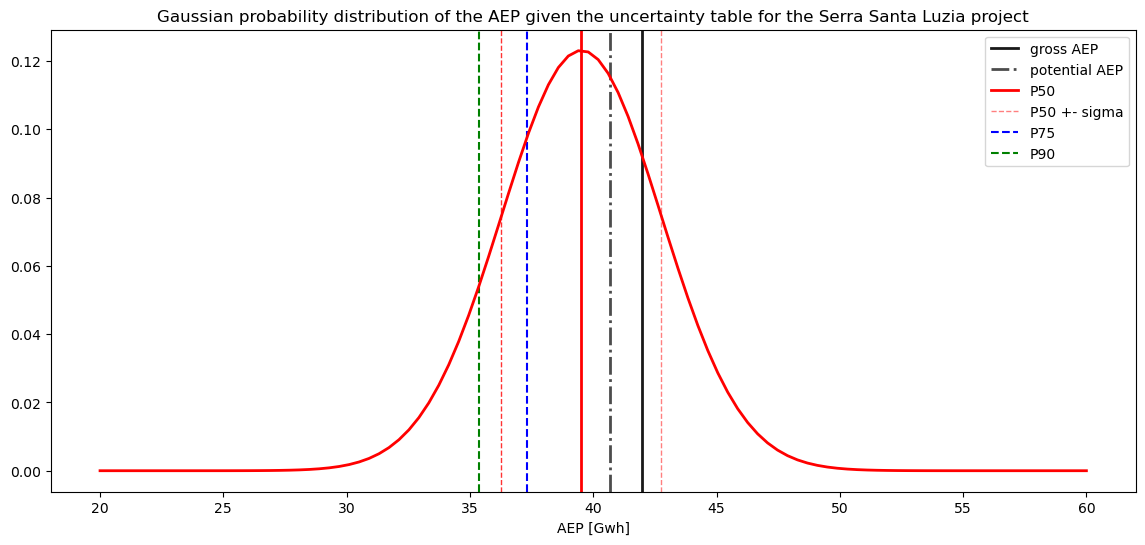
[18]:
# make a historgam of the real yields
from scipy.stats import norm

plt.figure(figsize=(14,6))

# now plot the pdf odf the normal distribution that we have estimatedusing scipy
x = np.linspace(20, 60, 100)

plt.axvline(gross_aep["gross_aep"].values.sum(), color='k', linestyle='-', alpha = 0.9 ,linewidth=2,label = "gross AEP")
plt.axvline(potential_aep["potential_aep"].values.sum(), color='k', linestyle='-.', alpha= 0.7, linewidth=2, label = "potential AEP")

plt.axvline(p50, color='r', linestyle='solid', linewidth=2, label="P50")
plt.axvline(p50+sigma_tot_dimensional, color='r', linestyle='dashed', linewidth=1, label="P50 +- sigma", alpha = 0.5)
plt.axvline(p50-sigma_tot_dimensional, color='r', linestyle='dashed', linewidth=1, alpha = 0.8)
plt.axvline(p90["P_75_aep"].values.sum(), color='b', linestyle='--', linewidth=1.5, label="P75")
plt.axvline(p90["P_90_aep"].values.sum(), color='g', linestyle='--', linewidth=1.5, label="P90")

pdf = norm.pdf(x, p50, sigma_tot_dimensional)

plt.plot(x, pdf, color='r', linewidth=2)

#legend
# plt.legend(["Real AEP mean", "","","gross_aep","potential_aep","P50","","", "P90"])
plt.legend()
plt.grid(visible= False)
plt.title("Gaussian probability distribution of the AEP given the uncertainty table for the Serra Santa Luzia project")
plt.xlabel("AEP [Gwh]")
plt.show()