PyWAsP: Importing objects from a WAsP workspace (WWH file)#
This tutorial covers a pywasp feature that lets users import objects from a WAsP workspace hierarchy (.wwh) file, and perform pywasp calculations with them. We will use the ‘Parque Ficticio’ workspace, which is also provided with the (Windows) WAsP GUI since version 11.
Based on the observed wind climate and its location given in this WWH, we will calculate site effects and predicted wind climates over a uniform grid, as was done in the first tutorial on resource grids.
After importing the necessary libraries, let’s read the wwh file and list its contents:
[1]:
import warnings
warnings.filterwarnings('ignore')  # We will ignore warnings to avoid cluttering the notebook

import windkit as wk
import pywasp as pw
import numpy as np
[2]:
wwh = wk.Workspace.read_wwh('./data/import/ParqueFicticio.wwh')
wwh
[2]:
 Object ID       Object description                               Object CRS
         3               Vector map {'elevation': 32719, 'roughness': 32719}
         6       Turbine site group                                       {}
        17 Generalised wind climate                                       {}
        19    Observed wind climate                                       {}
        22               Vector map {'elevation': 32719, 'roughness': 32719}
pywasp xarray datasets, by calling the corresponding wwh.get_ method and supplying the desired object id (possibly also with some additional parameters, depending on the object type). The first thing to notice is that we have two ID’s assigned to vector map objects. These two vector maps are identical, coming from a typical workspace where the vector map contains both roughness-change contours and elevation contours.WAsP to read the vector map in a specific way: one as an elevation map, and the other as a roughness map. As you will see later in this tutorial, we do this a bit differently in pywasp, compared to using WAsP’s GUI.NetCDF files, which are commonly used in meteorological applications and large wind atlases.Importing an OWC from the workspace#
Let’s start with the Observed wind climate. To get the OWC, we call the wwh method get_owc() and provide the id of this object:
[3]:
bwc = wwh.get_owc(19)
print(bwc)
<xarray.Dataset> Size: 4kB
Dimensions:       (point: 1, sector: 12, wsbin: 27)
Coordinates:
    height        (point) float64 8B 42.25
    south_north   (point) float64 8B 6.513e+06
    west_east     (point) float64 8B 2.622e+05
    crs           int8 1B 0
    wsceil        (wsbin) float64 216B 1.0 2.0 3.0 4.0 ... 24.0 25.0 26.0 27.0
    wsfloor       (wsbin) float64 216B 0.0 1.0 2.0 3.0 ... 23.0 24.0 25.0 26.0
    sector_ceil   (sector) float64 96B 15.0 45.0 75.0 ... 285.0 315.0 345.0
    sector_floor  (sector) float64 96B 345.0 15.0 45.0 ... 255.0 285.0 315.0
  * wsbin         (wsbin) float64 216B 0.5 1.5 2.5 3.5 ... 23.5 24.5 25.5 26.5
  * sector        (sector) float64 96B 0.0 30.0 60.0 90.0 ... 270.0 300.0 330.0
Dimensions without coordinates: point
Data variables:
    wdfreq        (sector, point) float64 96B 0.0706 0.0318 ... 0.1284 0.0883
    wsfreq        (wsbin, sector, point) float64 3kB 0.02467 ... 0.0002156
Attributes:
    Conventions:      CF-1.8
    history:          2025-07-04T13:13:16+00:00:\twindkit==1.0.0\tcreate_data...
    description:      Cerro
    Package name:     windkit
    Package version:  1.0.0
    Creation date:    2025-07-04T13:13:16+00:00
    Object type:      Binned Wind Climate
    author:           Bjarke Tobias Olsen
    author_email:     btol@dtu.dk
    institution:      DTU Wind
[4]:
bwc.to_netcdf('./data/export/bwc.nc')
Importing a GWC from the workspace#
In a similar fashion to the OWC, we import the Generalised wind climate, using the wwh.get_gwc method; we likewise export it to NetCDF file:
[5]:
gwc = wwh.get_gwc(17)
print(gwc)

gwc.to_netcdf('./data/export/gwc.nc')
<xarray.Dataset> Size: 8kB
Dimensions:        (point: 1, gen_height: 5, gen_roughness: 5, sector: 12)
Coordinates:
    height         (point) float64 8B 42.25
    south_north    (point) float64 8B 6.513e+06
    west_east      (point) float64 8B 2.622e+05
    crs            int8 1B 0
    sector_ceil    (sector) float64 96B 15.0 45.0 75.0 ... 285.0 315.0 345.0
    sector_floor   (sector) float64 96B 345.0 15.0 45.0 ... 255.0 285.0 315.0
  * gen_height     (gen_height) float64 40B 10.0 25.0 50.0 100.0 200.0
  * gen_roughness  (gen_roughness) float64 40B 0.0 0.03 0.1 0.4 1.5
  * sector         (sector) float64 96B 0.0 30.0 60.0 90.0 ... 270.0 300.0 330.0
Dimensions without coordinates: point
Data variables:
    A              (gen_height, gen_roughness, sector, point) float64 2kB 4.1...
    k              (gen_height, gen_roughness, sector, point) float64 2kB 1.7...
    wdfreq         (gen_height, gen_roughness, sector, point) float64 2kB 0.0...
Attributes:
    description:      Cerro
    Conventions:      CF-1.8
    Package name:     windkit
    Package version:  1.0.0
    Creation date:    2025-07-04T13:13:16+00:00
    Object type:      Weibull Wind Climate
    author:           Bjarke Tobias Olsen
    author_email:     btol@dtu.dk
    institution:      DTU Wind
    history:          2025-07-04T13:13:16+00:00:\twindkit==1.0.0\twwh.get_gwc...
Importing vector maps from the WAsP workspace#
Now let’s load the maps. To do this we call the method wwh.get_vectormap, which requires following parameters:
id: id of the vector map object in the wwh list (integer)srs: EPSG code of the mapmap_type: feature type to extract from mapfile, it can be ‘elevation’ or ‘roughness’
In our example the vector map header has following information: “UTM-Proj.-S.hemisph. Zone 19 (WGS 1984)”. This corresponds to an EPSG code of 32719. However, the output of pw.io.Workspace.read_wwh shows code 32619, because the header should say “…Zone19S…”.
maps note: One may need to examine map headers and ensure one knows the projection/datum (coordinates) of the map, or for locations within observed wind climate files. See the EPSG site to check coordinate systems. Sometimes one must look at map data and repeat reading it in, to transform coordinates properly.
We will extract both the elevation and roughness maps; we can use either ID (3 or 22). We will then bundle these two maps together using wasp.TopographyMap, which is needed for the various flow-perturbation calculations.
[6]:
elev_map = wwh.get_elevation_map(22, crs=32719)
rough_map = wwh.get_roughness_map(22, crs=32719)

topo_map = pw.wasp.TopographyMap(elev_map, rough_map)
If we closely inspect the OWC data (look at bwc.crs and click on check attributes or look at bwc.crs.crs_wkt), we notice that the provided geospatial location of the mast in this dataset is in coordinates following the EPSG:4326 projection (with south_north=latitude and west_east=longitude, i.e., in degrees not m).
However, as our terrain and rougness data are in UTM Zone 19S (EPSG:32719) we will convert and update the mast coordinates. Once the coordiantes are converted we will store them in in variables loc_x and loc_y for later use.
[7]:
bwc = wk.spatial.reproject(bwc, 32719)
loc_y = bwc.south_north
loc_x = bwc.west_east
(re-)calculating predicted wind climates#
creating a grid of locations#
Let’s first create uniform grid, with resolution of 100 m in west_east and north_south coordinate. The grid will be positioned 200 m above the ground level. We use pw.create_dataset to perform this.
[8]:
height = 200
x_res = 100
y_res = 100

output_locs = wk.spatial.create_dataset(
    np.arange(262878, 265078 + x_res, x_res),
    np.arange(6504214, 6507414 + y_res, y_res),
    np.array([height]),
    32719
)
calculating predicted wind climates over the grid#
Let’s now calculate predicted wind climate, site effects, and meteorological variables, using the pw.wasp.downscale routine. We will then export this to a NetCDF file:
[9]:
conf = pw.wasp.Config()
pwc = pw.wasp.downscale(gwc, topo_map, output_locs, conf, interp_method='nearest', return_site_effects=True)
print(pwc)
<xarray.Dataset> Size: 599kB
Dimensions:              (sector: 12, south_north: 33, west_east: 23, height: 1)
Coordinates:
    crs                  int8 1B 0
    sector_ceil          (sector) float64 96B 15.0 45.0 75.0 ... 315.0 345.0
    sector_floor         (sector) float64 96B 345.0 15.0 45.0 ... 285.0 315.0
  * height               (height) int64 8B 200
  * south_north          (south_north) int64 264B 6504214 6504314 ... 6507414
  * west_east            (west_east) int64 184B 262878 262978 ... 264978 265078
  * sector               (sector) float64 96B 0.0 30.0 60.0 ... 300.0 330.0
Data variables: (12/21)
    z0meso               (sector, south_north, west_east) float32 36kB 0.1 .....
    slfmeso              (sector, south_north, west_east) float32 36kB 1.0 .....
    displ                (sector, south_north, west_east) float32 36kB 0.0 .....
    flow_sep_height      (sector, south_north, west_east) float32 36kB 0.0 .....
    user_def_speedups    (sector, height, south_north, west_east) float32 36kB ...
    orographic_speedups  (sector, height, south_north, west_east) float32 36kB ...
    ...                   ...
    A                    (sector, height, south_north, west_east) float32 36kB ...
    k                    (sector, height, south_north, west_east) float32 36kB ...
    wdfreq               (sector, height, south_north, west_east) float32 36kB ...
    air_density          (height, south_north, west_east) float32 3kB 1.174 ....
    wspd                 (height, south_north, west_east) float32 3kB 7.428 ....
    power_density        (height, south_north, west_east) float32 3kB 459.6 ....
Attributes:
    Conventions:      CF-1.8
    history:          2025-07-04T13:13:17+00:00:\twindkit==1.0.0\twk.spatial....
    Package name:     windkit
    Package version:  1.0.0
    Creation date:    2025-07-04T13:13:19+00:00
    Object type:      Met fields
    author:           Bjarke Tobias Olsen
    author_email:     btol@dtu.dk
    institution:      DTU Wind
    title:            WAsP site effects
[10]:
pwc.to_netcdf('./data/export/results_'+str(height)+'_m.nc')
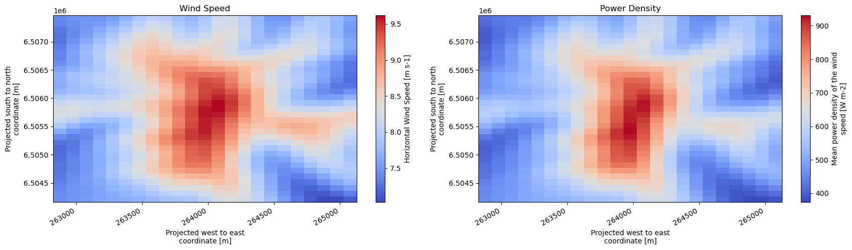
[11]:
import matplotlib.pyplot as plt
fig, axes = plt.subplots(1, 2, figsize=(17, 5))
ax1, ax2 = axes.flat
variables = ['wspd', 'power_density']
for var, ax in zip(variables, axes.flat):
    pwc[var].isel(height=0).plot(ax=ax, cmap='coolwarm')
    plt.setp(ax.get_xticklabels(), rotation=30, horizontalalignment='right')
ax1.set_title("Wind Speed")
ax2.set_title("Power Density");
fig.tight_layout()
Get turbine hub positions (x,y,z) from the workspace, and predict wind climates for them#
Finally let’s extract the positions of the wind turbines, and their hub height. To do this we use the wwh method get_turbines(). This method requires id and srs as inputs, and generates an xarray dataset containing the positions of wind turbines:
[12]:
wtg_pos = wwh.get_turbines(6, 32719)
print(wtg_pos)
<xarray.Dataset> Size: 257B
Dimensions:      (point: 8)
Coordinates:
    height       (point) float64 64B 70.0 70.0 70.0 70.0 70.0 70.0 70.0 70.0
    south_north  (point) float64 64B 6.505e+06 6.505e+06 ... 6.506e+06 6.507e+06
    west_east    (point) float64 64B 2.639e+05 2.64e+05 ... 2.639e+05 2.637e+05
    crs          int8 1B 0
Dimensions without coordinates: point
Data variables:
    output       (point) float64 64B 0.0 0.0 0.0 0.0 0.0 0.0 0.0 0.0
Attributes:
    Conventions:  CF-1.8
    history:      2025-07-04T13:13:20+00:00:\twindkit==1.0.0\t        return ...
Now we can calculate and see what the power densities look like at the turbine sites:
[13]:
pwc_wtgs = pw.wasp.downscale(gwc, topo_map, wtg_pos, conf, interp_method='nearest', return_site_effects=True)
[14]:
print(pwc_wtgs.power_density.values)
[573.2814  640.4514  664.58826 608.77576 656.47925 621.65656 514.6878
 425.05362]
Quick question: why do these power densities seem much lower than the ones in the plot further above? (hint: what is different between output_locs and wtg_pos?)