Generalized wind climate interpolation#
This notebook shows some examples of interpolating different generalized or geostrophic wind climate that you may have obtained from masts or numerical weather prediction model output. All the main flow prediction functions (e.g. downscale, downscale_from_site_effects) have a argument interp_method. The default of this argument is nearest, because it always returns a result. However, there might be better ways of interpolating your GWC’s. This tutorial will help you understand
how this argument is influencing your results when you have more than one GWC to predict over a certain area. Under the hood, pywasp will use the method pw.wasp.interpolate_gwc as explained below.
[1]:
import pywasp as pw
import windkit as wk
import numpy as np
import itertools
import matplotlib.pyplot as plt
import time
import pandas as pd
Prepare Generalized Wind climate cuboid#
Let’s say we have a grid of generalized wind climates from the WRF model. In the code below we make a cuboid in a certain area of 90km x 90km covered by nr_grid_points (4 in each direction). This area is just filled with random data using the create_gwc method. We apply a running mean to the grid cells to get some coherence between the pixels, so that interpolation is more similar as a real WRF grid, where the pixels will mostly have quite slowly varying mean wind speeds.
[2]:
def gwc_cuboid(nr_grid_points=4):
    gwc_locs = wk.spatial.create_cuboid(
        np.linspace(620000, 710000, nr_grid_points),
        np.linspace(6090000, 6180000, nr_grid_points),
        height=100.0,
        crs="EPSG:32632",
    )

    gwc = wk.create_gwc(gwc_locs, seed=0)
    gwc = gwc.rolling(west_east=nr_grid_points // 2, min_periods=1, center=True).mean()
    gwc = gwc.rolling(
        south_north=nr_grid_points // 2, min_periods=1, center=True
    ).mean()
    return gwc
If you are using a more modern wind atlas you may similarly have a grid of geostrophic wind climates. For example NEWA v2 and the GWA version 4 were run with these outputs. Geostrophic wind climate have various advantages over generalized wind climates, most importantly it’s ability to better retain information about the mean wind speed in each sector. They have a variable geo_wv_freq, which represents the geostrophic wind speed frequency by wind direction and wind speed. In addition, it has
the variable geo_turn, which is needed to interpolate geostrophic turning which is needed for transforming the wind direction frequency as a function of height and mesoscale roughness length. Finally, more information about how the generalization was done is required, because the roughness length, the height and the sea-land fraction are used in in the stability model in the downscaling step.
[3]:
def geowc_cuboid(nr_grid_points=4):
    gwc_locs = wk.spatial.create_cuboid(
        np.linspace(620000, 710000, nr_grid_points),
        np.linspace(6090000, 6180000, nr_grid_points),
        height=100.0,
        crs="EPSG:32632",
    )
    gwc = wk.create_geowc(gwc_locs, seed=0, n_wsbins=60, n_sectors=4)
    gwc = gwc.rolling(west_east=nr_grid_points // 2, min_periods=1, center=True).mean()
    gwc = gwc.rolling(
        south_north=nr_grid_points // 2, min_periods=1, center=True
    ).mean()

    return gwc
GWC interpolation for the windkit spatial structures#
We may want to use these GWC’s to downscale over an area that is covered by several of the grid cells in the GWC cuboid. This area can have all windkit spatial structures: you may have some masts (stacked point/point) or a regular WRF output grid with a cuboid structure. To illustrate the methods for these scenarios below we are making the product of all possible combinations. We can then apply 3 interpolation strategies to the data: nearest, linear or natural. You can read more about these interpolation methods on the scipy https://docs.scipy.org/doc/scipy/tutorial/interpolate.html
Irregular grids (stacked_point or point) are interpolated using the interpolators listed under the N-D scattered entries on the above page.
If your input GWC’s are in a regular grid (cuboid structure) the RegularGridInterpolator is used under the hood. This avoids the computationally expensive triangulation that is needed for unstructured grid.
[4]:
methods = [
    "nearest",
    "linear",
    "natural",
]

spatial_structs = [
    "point",
    "stacked_point",
    "cuboid",
]

all_combinations = list(itertools.product(methods, spatial_structs, spatial_structs))

input_structs = target_structs = spatial_structs
We may want to use these GWC’s to downscale over an area that is covered by some or all of the grid cells in the GWC cuboid. This area can have several spatial structures: you may have some masts (irregular points) or a resource grid with a fine resolution (regular cuboid structure).
To have a realistic example we select only 3 GWC locations, to mimic the case where we have GWC’s from some masts or met towers to downscale from. while for the meso-scale model case we will use a cuboid structure of 4x4 grid points. The stacked_point input will also share the later, thus being 16 stacked points in total.
In addition also the output spatial structure may be either point, stacked_point or cuboid. In the script below the output locations always have a cuboid structure, because it is easier to visualize. Although the stacked point and cuboid output structures are specified at the same output locations, the stacked point structure results in a different code path that uses a different interpolator (unstructured vs structured). This can be seen as subtle differences in the output wind
climates, as shown in the plots below.
These scenarios are simulated below by making the product of all combinations possible. We can then apply 3 interpolation strategies to the data: nearest, linear or natural. The scenarios have been made only with generalized wind climate (GWC) as input for simplicity, but the user is encouraged to make use of the geowc_cuboid() function if desired by changing the line under # GWC data preparation.
Nearest neighbour interpolation is fast but may introduce artifacts in the output wind climate. Linear interpolation is a good compromise between speed and quality.
Note
The natural neighbor interpolation is only supported for point output structures in this example. It will be skipped for other output structures. Also note that some warnings from the natural neighbour interpolation are resulting from running the plots below, as it cannot understand what to do outside the convex hull of the input points. This is the correct behavior.
When using linear interpolation with point input structures (unstructured data), the method relies on triangulation. Points outside the convex hull of the input locations cannot be interpolated and will result in NaN values (shown as white/empty areas in the plots). Nearest neighbor interpolation does not have this limitation and will extrapolate to cover the full domain.
[5]:
timings = {}

# Create figure per input structure
vmin, vmax = 5.0, 8.5
figs = {}
axes = {}
for in_struct in input_structs:
    fig, axs = plt.subplots(
        nrows=len(methods),
        ncols=len(target_structs),
        figsize=(20, 18),
        sharex=True,
        sharey=True,
    )
    figs[in_struct] = fig
    axes[in_struct] = axs

    # Figure title (input structure)
    fig.suptitle(f"GWC input structure: {in_struct}", fontsize=22, weight="bold")

    # Column headers (output structures)
    for j, out_struct in enumerate(target_structs):
        axs[0, j].set_title(
            out_struct.replace("_", " ").capitalize(), fontsize=16, pad=14
        )

# Fill subplots
for method, in_struct, out_struct in all_combinations:
    fig_key = in_struct
    i = methods.index(method)
    j = target_structs.index(out_struct)
    ax = axes[fig_key][i, j]

    # Skip unavailable case (natural + non-point output)
    if out_struct != "point" and method == "natural":
        ax.set_facecolor("#f0f0f0")
        ax.text(
            0.5,
            0.5,
            "Not available\nfor this case",
            ha="center",
            va="center",
            fontsize=14,
            color="red",
            transform=ax.transAxes,
        )
        ax.set_xticks([])
        ax.set_yticks([])
        continue

    # GWC data preparation
    gwc = gwc_cuboid(4).copy()
    var = "A" if "A" in gwc.data_vars else "geo_wv_freq"

    # Target grid based on GWC extent
    bbox = wk.spatial.BBox.from_ds(gwc)
    output_locs = bbox.buffer(7000).to_grid(spacing=5000.0, heights=[0.0])

    # Convert output structure
    if out_struct == "point":
        output_locs = wk.spatial.to_point(output_locs)
    elif out_struct == "stacked_point":
        output_locs = wk.spatial.to_stacked_point(output_locs)

    # Convert input structure
    if in_struct == "point":
        gwc = wk.spatial.to_point(gwc).isel(point=[0, 3, 15])
    elif in_struct == "stacked_point":
        gwc = wk.spatial.to_stacked_point(gwc)

    # Interpolation
    t = time.process_time()
    gwc_out = pw.wasp.interpolate_gwc(
        gwc, output_locs, method=method, engine="windkit", fill_value=np.nan
    )
    timings[(method, in_struct, out_struct)] = time.process_time() - t

    # Convert to cuboid for plotting
    gwc_cubic = wk.spatial.to_cuboid(gwc_out)
    if wk.is_gwc(gwc_out):
        gwc_cubic = gwc_cubic.isel(gen_roughness=2, gen_height=2)

    # Compute mean wind speed
    mean_ws = wk.mean_wind_speed(gwc_cubic, bysector=True).isel(sector=0).squeeze()

    # Plot
    im = mean_ws.plot.pcolormesh(
        x="west_east", y="south_north", ax=ax, add_colorbar=False, vmin=vmin, vmax=vmax
    )
    wk.spatial.ds_to_gdf(gwc).plot(ax=ax, marker="x", color="black", markersize=30)
    ax.set_title(f"interp: {method} → {out_struct}", fontsize=20, pad=6)
    ax.set_xticks([])
    ax.set_yticks([])

# Colorbars & layout
for in_struct, fig in figs.items():
    cbar_ax = fig.add_axes([0.92, 0.15, 0.015, 0.7])
    cbar = fig.colorbar(im, cax=cbar_ax)
    cbar.set_label("Mean wind speed [m/s]", fontsize=16)
    for ax in fig.axes:
        for label in ax.get_xticklabels() + ax.get_yticklabels():
            label.set_fontsize(14)
    fig.tight_layout(rect=[0, 0, 0.9, 1], pad=3)
/home/neil/DTU/repos/pywasp/pywasp/wasp/generalized_wind_climate.py:303: UserWarning: Generalized wind climate interpolation resulted in NaN's. Use fill_value=None to fill these data with the nearest values.
  warnings.warn(
/home/neil/DTU/repos/pywasp/pywasp/wasp/generalized_wind_climate.py:303: UserWarning: Generalized wind climate interpolation resulted in NaN's. Use fill_value=None to fill these data with the nearest values.
  warnings.warn(
/home/neil/DTU/repos/pywasp/pywasp/wasp/generalized_wind_climate.py:303: UserWarning: Generalized wind climate interpolation resulted in NaN's. Use fill_value=None to fill these data with the nearest values.
  warnings.warn(
/home/neil/DTU/repos/pywasp/pywasp/wasp/generalized_wind_climate.py:303: UserWarning: Generalized wind climate interpolation resulted in NaN's. Use fill_value=None to fill these data with the nearest values.
  warnings.warn(
/home/neil/DTU/repos/pywasp/pywasp/wasp/generalized_wind_climate.py:303: UserWarning: Generalized wind climate interpolation resulted in NaN's. Use fill_value=None to fill these data with the nearest values.
  warnings.warn(
/home/neil/DTU/repos/pywasp/pywasp/wasp/generalized_wind_climate.py:303: UserWarning: Generalized wind climate interpolation resulted in NaN's. Use fill_value=None to fill these data with the nearest values.
  warnings.warn(
/home/neil/DTU/repos/pywasp/pywasp/wasp/generalized_wind_climate.py:303: UserWarning: Generalized wind climate interpolation resulted in NaN's. Use fill_value=None to fill these data with the nearest values.
  warnings.warn(
/home/neil/DTU/repos/pywasp/pywasp/wasp/generalized_wind_climate.py:303: UserWarning: Generalized wind climate interpolation resulted in NaN's. Use fill_value=None to fill these data with the nearest values.
  warnings.warn(
/home/neil/DTU/repos/pywasp/pywasp/wasp/generalized_wind_climate.py:303: UserWarning: Generalized wind climate interpolation resulted in NaN's. Use fill_value=None to fill these data with the nearest values.
  warnings.warn(
Error during processing of a grid. Interpolation will continue but be mindful of errors in output. Circumcenter calculation failed due to division by zero.
Error during processing of a grid. Interpolation will continue but be mindful of errors in output. Circumcenter calculation failed due to division by zero.
Error during processing of a grid. Interpolation will continue but be mindful of errors in output. Circumcenter calculation failed due to division by zero.
Error during processing of a grid. Interpolation will continue but be mindful of errors in output. Circumcenter calculation failed due to division by zero.
Error during processing of a grid. Interpolation will continue but be mindful of errors in output. Circumcenter calculation failed due to division by zero.
Error during processing of a grid. Interpolation will continue but be mindful of errors in output. Circumcenter calculation failed due to division by zero.
Error during processing of a grid. Interpolation will continue but be mindful of errors in output. Circumcenter calculation failed due to division by zero.
Error during processing of a grid. Interpolation will continue but be mindful of errors in output. Circumcenter calculation failed due to division by zero.
Error during processing of a grid. Interpolation will continue but be mindful of errors in output. Circumcenter calculation failed due to division by zero.
Error during processing of a grid. Interpolation will continue but be mindful of errors in output. Circumcenter calculation failed due to division by zero.
Error during processing of a grid. Interpolation will continue but be mindful of errors in output. Circumcenter calculation failed due to division by zero.
Error during processing of a grid. Interpolation will continue but be mindful of errors in output. Circumcenter calculation failed due to division by zero.
Error during processing of a grid. Interpolation will continue but be mindful of errors in output. Circumcenter calculation failed due to division by zero.
Error during processing of a grid. Interpolation will continue but be mindful of errors in output. Circumcenter calculation failed due to division by zero.
Error during processing of a grid. Interpolation will continue but be mindful of errors in output. Circumcenter calculation failed due to division by zero.
Error during processing of a grid. Interpolation will continue but be mindful of errors in output. Circumcenter calculation failed due to division by zero.
Error during processing of a grid. Interpolation will continue but be mindful of errors in output. Circumcenter calculation failed due to division by zero.
Error during processing of a grid. Interpolation will continue but be mindful of errors in output. Circumcenter calculation failed due to division by zero.
/home/neil/DTU/repos/pywasp/pywasp/wasp/generalized_wind_climate.py:303: UserWarning: Generalized wind climate interpolation resulted in NaN's. Use fill_value=None to fill these data with the nearest values.
  warnings.warn(
/home/neil/DTU/repos/pywasp/pywasp/wasp/generalized_wind_climate.py:303: UserWarning: Generalized wind climate interpolation resulted in NaN's. Use fill_value=None to fill these data with the nearest values.
  warnings.warn(
/home/neil/DTU/repos/pywasp/pywasp/wasp/generalized_wind_climate.py:303: UserWarning: Generalized wind climate interpolation resulted in NaN's. Use fill_value=None to fill these data with the nearest values.
  warnings.warn(
/tmp/ipykernel_2693638/737036618.py:98: UserWarning: Adding colorbar to a different Figure <Figure size 2000x1800 with 9 Axes> than <Figure size 2000x1800 with 10 Axes> which fig.colorbar is called on.
  cbar = fig.colorbar(im, cax=cbar_ax)
/tmp/ipykernel_2693638/737036618.py:103: UserWarning: This figure includes Axes that are not compatible with tight_layout, so results might be incorrect.
  fig.tight_layout(rect=[0, 0, 0.9, 1], pad=3)
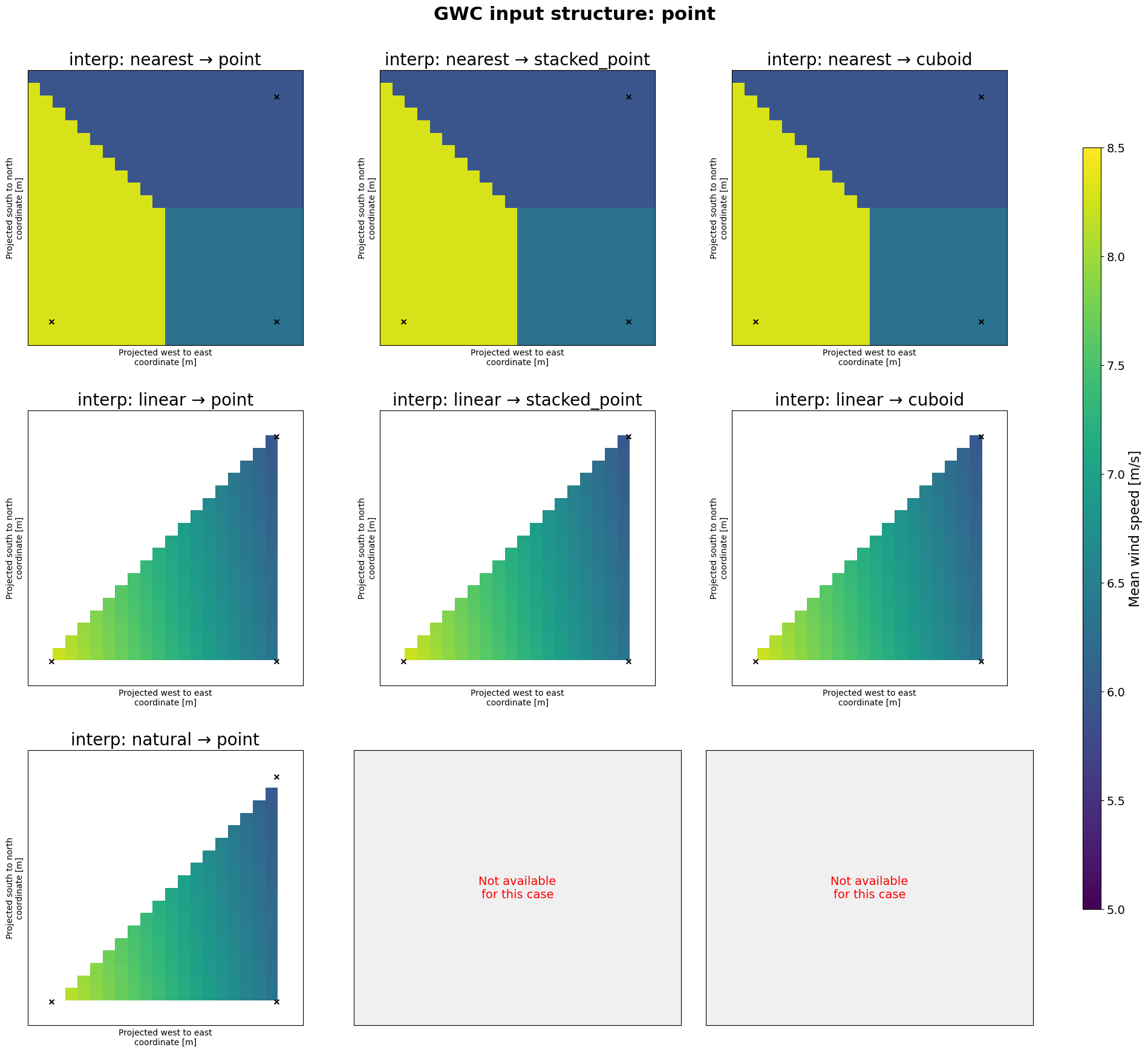
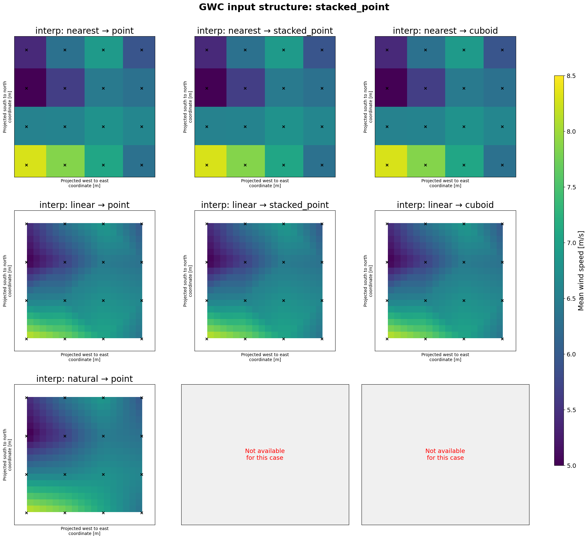
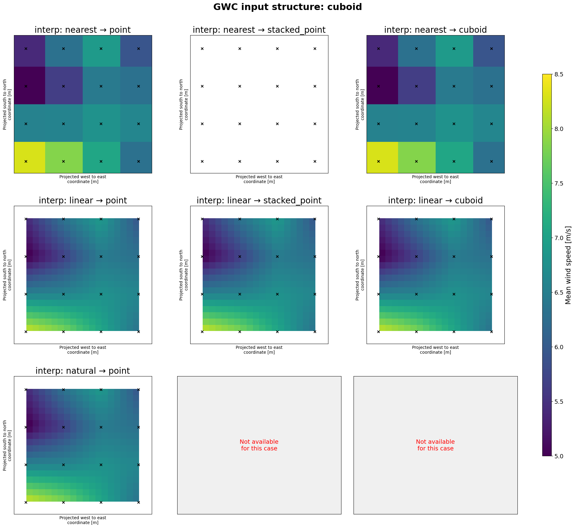
Using the argument fill_value=None in the above does an additional interpolation in the data to fill requested points that are outside the area contained in the GWC’s using nearest neighbour interpolation. Setting it to the fill_value=np.nan leaves those points as nan’s. Also notice how artifacts from the triangulation are visible when interpolating from unstructured grids.
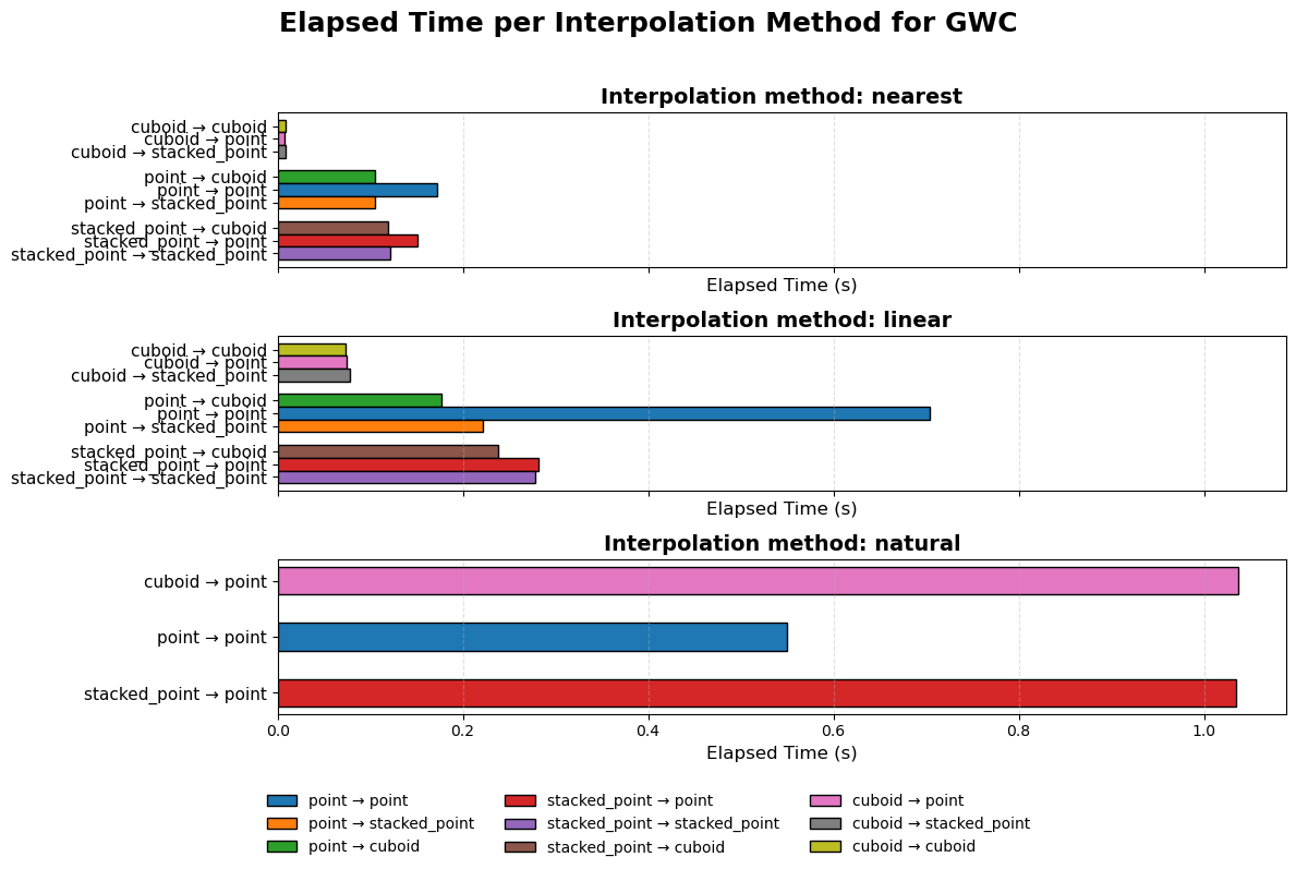
Performance#
The performance of the different methods is shown below. The natural neighbour interpolation is the most expensive and takes quite long even for smaller grids. The other methods perform better. When the input is structured (cuboid) the performance is quite a bit better as no triangulation has to be done. The performance of geostrophic wind climate linear interpolation is quite good in this case, but may suffer when the dimensions (all spatial dimension plus the number of wind speed bins and sectors, i.e. 5D interpolation) grow. Initially there was some code that was calculating the moments, interpolating those and then remapping the geostrophic wind climates. This has now been removed, but may have to be reintroduced when simulating wind atlasses, where the grids can be substantially bigger.
[6]:
# Prepare DataFrame
df = pd.DataFrame(
    {"elapsed time": timings.values()}, index=pd.MultiIndex.from_tuples(timings.keys())
)
df = df.reset_index()
df.columns = ["method", "input_struct", "output_struct", "elapsed time"]

# Combined key for consistent color assignment
df["combination"] = df[["input_struct", "output_struct"]].apply(
    lambda r: f"{r.iloc[0]} → {r.iloc[1]}", axis=1
)

# Define colors for each input→output combination
unique_combos = df["combination"].unique()
cmap = plt.colormaps["tab10"]  # use distinct colors
combo_colors = {combo: cmap(i) for i, combo in enumerate(unique_combos)}

# Plot Configuration
bar_height = 0.8
group_gap = 0.8

methods = df["method"].unique()
num_methods = len(methods)
fig, axes = plt.subplots(nrows=num_methods, ncols=1, figsize=(12, 8), sharex=True)

# Generate Subplots per interpolation method
for i, method in enumerate(methods):
    ax = axes[i] if num_methods > 1 else axes
    df_subset = df[df["method"] == method].sort_values(
        ["input_struct", "output_struct"]
    )

    y_ticks = []
    y_labels = []
    current_y = 0

    # Group by input structure for visual clarity
    for input_struct, group in df_subset.groupby("input_struct"):
        group = group.sort_values("output_struct")

        for _, row in group.iterrows():
            combo = row["combination"]
            color = combo_colors[combo]

            ax.barh(
                y=current_y,
                width=row["elapsed time"],
                height=bar_height,
                color=color,
                edgecolor="black",
            )
            y_ticks.append(current_y)
            y_labels.append(combo)
            current_y += bar_height

        current_y += group_gap

    # Axis settings
    ax.set_yticks(y_ticks)
    ax.set_yticklabels(y_labels, fontsize=11)
    ax.set_title(f"Interpolation method: {method}", fontsize=14, weight="bold")
    ax.set_xlabel("Elapsed Time (s)", fontsize=12)
    ax.invert_yaxis()
    ax.grid(axis="x", linestyle="--", alpha=0.4)

# Add a legend for combinations
handles = [
    plt.Rectangle((0, -1.5), 1, 1, color=c, ec="black") for c in combo_colors.values()
]
fig.legend(
    handles, combo_colors.keys(), loc="lower center", ncol=3, fontsize=10, frameon=False
)

# Overall Figure Layout
fig.suptitle(
    "Elapsed Time per Interpolation Method for GWC", fontsize=18, weight="bold"
)
fig.tight_layout(rect=[0, 0.1, 1, 0.96])
Case study using WRF data#
To investigate the real world impact of interpolation of generalized wind climates we can use the NEWA WRF output. We select points every 2nd grid cell where we generalize the binned wind climate (red points) and try to predict an adjacent but different grid cells (green points). We use the original WRF grid roughness length and elevation for both the generalization and downscaling. We can then compare the downscaled wind climate at the green points with the observed wind climate from the WRF model, thereby investigating how big errors we are making in the interpolation.

Looking at the figure below, it is clear that the largest errors occur in the Alps, where there are large differences due to orographic speedups. In flat terrain the errors are very close to zero.

We now look at the whole central europe domain in the NEWA, following the approach above. We can compare the three methods discussed before (nearest, linear and natural) and also apply both the generalization that is using the generalized wind climate as intermediate wind climate, but also the geostrophic wind climate. Furthermore we look at both variables wind speed and power density. First looking at the first 4 methods ending with geo (for geostrophic wind climate as intermediate format), it
can be seen in the figure below that for the method nearest the mean errors (expressed as percentage) are larger than for linear and natural.
Furthermore, it can be seen that using the linear unstructured interpolation performs slighlty worse than the normal (structured) linear interpolation. This can be because the unstructured interpolation only use the 3 nearest grid points, whereas the structured interpolation can use the information from the nearest 4 grid points.
Looking at the last 6 entries, similar conclusions can be drawn for the normal generalization (using generalized wind climates. For comparison the results from the now deprecated fortran engine that were used for GWA3 are also shown. The nearest method again has the highest errors. linear and natural perform very similarly and the unstructured interpolation has again somewhat higher errors.

Finally we can take a brief look at the distributions in wind speed errors. As example we look at the relative errors in percent for the structured linear method and compare the generalized (GWC) with the geostrophic wind climate (GeoWC). For the graph below it is quite obvious that using the geostrophic wind climate generally results in errors that are closer to 0.
