Classical resource assessment step-by-step#
Introduction#
The example works through a complete wind turbine siting operation, starting with some measured wind data and ending up with a prediction of the power yield by erecting wind turbies at a specific site. This example includes AEP calculation which consider wake losses. You will set up a wind farm consisting of several wind turbines and predict the annual energy production from this farm. Finally, we’ll map the wind resource over an area.
pywasp note:
pywasprelies on the wake models from PyWake and park2 to calculate energy losses caused by the rotor wakes. PyWake is installed with PyWAsP, so you should be ready to go. If not, you can install PyWake from a conda enviroment containingpywaspby execute following command in a terminalpip install git+https://gitlab.windenergy.dtu.dk/TOPFARM/cuttingedge/pywake/pywake_park.git
The situation#
The company Friends of Wind Energy, E-Corp Ltd. has asked you to provide a prediction of the power yield from locating a wind turbine in Serra Santa Luzia area in Portugal. They propose to erect a single 1-MW wind turbine at the summit of Serra Santa Luzia hill (they have modest energy requirements).
No wind measurements have been taken at the turbine site itself, but data have been collected from a meteorological station at nearby hill.
You are equipped with:
a contour map of the area
the wind data from the met station
a simple description of the land cover in the area
a description of the power-generating characteristics of the turbine
These data are located in the data subfolder as following files:
a digital map of elevations and roughness
SerraSantaLuzia.mapa file containing wind data
SerraSantaLuzia.omwca data file containing a power production curve for the turbine
Bonus_1_MW.wtg
Working with WAsP to provide a prediction#
From engineering data, you know how much power will be generated by the turbine at a given wind speed. If the plan was to erect the turbine at exactly the same place where the meteorological data had been collected, then it would be a really simple task to work out how much power to expect.
However, just from looking at the map it is obvious that the proposed turbine site is completely different from the meteorological station at the airport: the properties of the meteorological station itself will affect the wind data recorded there. In addition, the properties of the turbine site will have an effect on the way that the wind behaves near the turbine. It is also unlikely that the hub height of the turbine would be the same as the height of the anemometer.
What you need is a way to take the wind climate recorded at the meteorological station, and use it to predict the wind climate at the turbine site. That is what pywasp does.
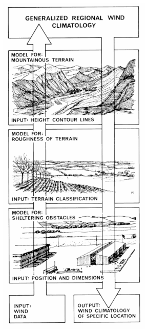
Using pywasp, you can analyse the recorded wind data, correcting for the recording site effects to produce a site-independent characterization of the local wind climate. This site-independent characterization of the local wind climate is called a wind atlas data set or generalised wind climate. You can also use pywasp to apply site effects to generalised wind climate data to produce a site-specific interpretation of the local wind climate.
Providing a prediction in the Waspdale case will therefore be a two-stage process (depicted in the right image). First, the data from the meteorological station need to be analysed to produce a wind atlas (“going up” in WAsP lingo), and then the resulting generalised wind climate needs to be applied to the proposed turbine site to estimate the wind power (“going down” in WAsP lingo).
Import packages#
Usually the first step when writing a python program is importing standard and external packages we will need. For this analysis we will import numpy, pandas, matplotlib, xarray, pywasp, pywake and PARK pywake plugin.
numpyis python’s main numerical array package https://www.numpy.org/pandasis python’s main package for manipulation of tabular data https://pandas.pydata.org/matplotlibis python’s main plotting package https://matplotlib.org/xarrayis a powerful high level package for labelled multi-dimensional arrays http://xarray.pydata.orgpywaspdocummentation is found at http://docs.wasp.dk/py_wakedocummentation is found at https://topfarm.pages.windenergy.dtu.dk/PyWake/py_wake_parkdocummentation is found at https://gitlab.windenergy.dtu.dk/TOPFARM/cuttingedge/pywake/pywake_park
As you work your way through the notebook, make sure to run the python code in each cell in the order that they appear. You run the code by clicking on the cell (outlines around the cell should appear) and pressing <shift> + <enter> on the keyboard.
notebook note: if something looks wrong, or when errors occur, it can be helpful to restart the python kernel via the kernel tab in the top
[1]:
%load_ext autoreload
%autoreload 2
import warnings

import numpy as np
import pandas as pd
import matplotlib.pyplot as plt

import windkit as wk
import pywasp as pw

warnings.filterwarnings("ignore")  # We will ignore warnings to avoid cluttering the notebook
It is common to make a short alias of the package when importing using the import - as - syntax. The functions and classes of imported packages must be accessed through explicitly typing the package name or alias, e.g. np.cos(3.14) will use the cosine function from numpy.
Observed wind climate#
Now we will import our (observed) binned wind climate from the mast located at hill nearby Serra Santa Luzia hill where the turbine is going to be installed. As mentioned earlier, the binned wind climates is stored in SerraSantaLuzia.omwc in the data folder. It represents the observed wind climate for the period
1997-2002 at 25.3 m above ground level.
pywasp note
pywaspincludes functionality to both read and write wind climate files in many data formats, including ascii (.tab), xml (.owcand.omwc), and netCDF (.nc).
The geospatial coordinate in the file is in the World Geodetic System 1984, (EPSG:4326), better known as a simple latitude/longitude. When possible, the file readers will try to parse the coordinate reference system (CRS). We can tell pywasp this by explicitly passing the keyword argument crs=4326 to the open_bwc.
[2]:
bwc = wk.read_bwc('./data/SerraSantaLuzia.omwc')
print(bwc)
<xarray.Dataset> Size: 4kB
Dimensions:       (point: 1, sector: 12, wsbin: 32)
Coordinates:
    height        (point) float64 8B 25.3
    south_north   (point) float64 8B 41.74
    west_east     (point) float64 8B -8.823
    crs           int8 1B 0
    wsceil        (wsbin) float64 256B 1.0 2.0 3.0 4.0 ... 29.0 30.0 31.0 32.0
    wsfloor       (wsbin) float64 256B 0.0 1.0 2.0 3.0 ... 28.0 29.0 30.0 31.0
    sector_ceil   (sector) float64 96B 15.0 45.0 75.0 ... 285.0 315.0 345.0
    sector_floor  (sector) float64 96B 345.0 15.0 45.0 ... 255.0 285.0 315.0
  * wsbin         (wsbin) float64 256B 0.5 1.5 2.5 3.5 ... 28.5 29.5 30.5 31.5
  * sector        (sector) float64 96B 0.0 30.0 60.0 90.0 ... 270.0 300.0 330.0
Dimensions without coordinates: point
Data variables:
    wdfreq        (sector, point) float64 96B 0.05314 0.03321 ... 0.1148 0.0707
    wsfreq        (wsbin, sector, point) float64 3kB 0.02601 0.04219 ... 0.0 0.0
Attributes:
    Conventions:      CF-1.8
    history:          2025-07-04T13:07:08+00:00:\twindkit==1.0.0\tcreate_data...
    description:      SerraSantaluzia
    Package name:     windkit
    Package version:  1.0.0
    Creation date:    2025-07-04T13:07:08+00:00
    Object type:      Binned Wind Climate
    author:           Bjarke Tobias Olsen
    author_email:     btol@dtu.dk
    institution:      DTU Wind
Notice that the bwc object is of type <xarray.Dataset> and that it contains four kinds of data:
Dimensions: core named dimensions
Coordinates: coordinate values along dimensions
Data variables: named arrays with data along 0-N named dimensions
Attributes: additional meta data attached to the dataset
xarray note the primitive datatype and dimensions of each variable are also shown, along with a small sample of the data.
wsfreqis a four-dimensionalfloat64(double precision) variable along dimensions(wsbin, sector, height, point)
Xarray datasets wrap numpy arrays, annotating them with human-readable dimensions and coordinates, and allowing for easy subsetting, data manipulation, and plotting of the underlying data. An xarray.Dataset object is a collection of data variables, while each varible itself has type xarray.DataArray.
xarray note Use the
.valuesobject attribute to access the underlying numpy array
Beyond the wind speed and wind direction distributions, the wind climate contains information about the height of the measurements (height) and the geospatial location (west_east and south_north), which in this case hold the location information in the projected coordinates of the EPSG:4326 projection (i.e., south_north=latitude and west_east=longitude). However, as our terrain and rougness data are in the UTM Zone 29 (EPSG:32629) we could convert and update
the mast coordinates explicitly by using bwc = wk.spatial.reproject(bwc, "EPSG:32629"). This is not strictly needed usually, because the bwc will be automatically reprojected to the coordinate system of the map. However, here the coordiantes are converted because we will store them in in variables loc_x and loc_y for later use.
[3]:
bwc = wk.spatial.reproject(bwc, "EPSG:32629")
loc_y = bwc.south_north
loc_x = bwc.west_east
The next step is to plot the wind rose and wind speed distributions in the binned wind climate.
notebook note: you can view the documentation for a function in jupyter notebooks by placing a
?in front of the function, and you can get the entire function by using??.
[4]:
wk.plot.histogram_lines(bwc)
Data type cannot be displayed: application/vnd.plotly.v1+json
As expected the prevailing wind direction at the site is from west (from the Atlantic ocean).
Topography data#
Now that we have loaded and inspected the wind climate, the next step is to the same with the terrain and roughness data. These data are used to calculate site effects used to generalize the observed wind climate (“going up” in WAsP lingo) and to downscale to nearby locations (“going down”).
The site effects are:
Orographic speed-up (by sector)
Internal boundar layer speed-up (by sector)
Effective upstream surface roughness (by sector)
pywasp note WAsP includes site effects due to obstacles, but we will not consider those here
Conveniently the terrain and roughness data are provided as a single vector map SerraSantaLuzia.map. To load data we will use wk.read_roughness_map() whereas for the elevation data we can use wk.read_elevation_map().
Creating topography map#
The elevation and roughness maps are the two components needed to make a TopographyMap object in pywasp, which is used to calculate the terrain effects.
In PyWAsP roughness map’s are automatically converted to a land cover maps with land cover id’s and roughness (z0) and displacement (d) values.
[5]:
elev_map = wk.read_elevation_map("data/SerraSantaLuzia.map")

landcover_map = wk.read_roughness_map(
    "data/SerraSantaLuzia.map",
    crs="EPSG:32629"
)

topo_map = pw.wasp.TopographyMap(elev_map, landcover_map)
Landcover maps in WAsP are characterized by polygons, that denotes the properties of a certain type of landcover. The properties used are roughness (z0), and optionally a displacement height (d) and description (desc).
[6]:
landcover_map
[6]:
| id | geometry | z0 | d | desc | |
|---|---|---|---|---|---|
| 0 | 0.0 | POLYGON ((520129.5 4608000, 520157.1 4608018.5... | 0.03 | 0.0 | |
| 1 | 0.0 | POLYGON ((520157.1 4608018.5, 520129.5 4608000... | 0.03 | 0.0 | |
| 2 | 0.0 | POLYGON ((522602.4 4608000, 522613.5 4608058, ... | 0.03 | 0.0 | |
| 3 | 1.0 | POLYGON ((522613.5 4608058, 522602.4 4608000, ... | 0.60 | 0.0 | |
| 4 | 1.0 | POLYGON ((518024.6 4608000, 518062.3 4608074.5... | 0.60 | 0.0 | |
| ... | ... | ... | ... | ... | ... |
| 338 | 5.0 | POLYGON ((525157.1 4637000, 525155.9 4636996.5... | 0.10 | 0.0 | |
| 339 | 1.0 | POLYGON ((526041.6 4637000, 526024.6 4636974, ... | 0.60 | 0.0 | |
| 340 | 0.0 | POLYGON ((512276.3 4637000, 512271.8 4636986, ... | 0.03 | 0.0 | |
| 341 | 1.0 | POLYGON ((524201 4636832.5, 524152.8 4636863, ... | 0.60 | 0.0 | |
| 342 | 4.0 | POLYGON ((509780.5 4637000, 509768.8 4636924, ... | 0.00 | 0.0 |
343 rows × 5 columns
Displaying terrain and roughness data#
To display the elevation roughness we can call wk.plot.elevation_map and wk.plot.landcover_map. These are plotting functions form windkit that use some default color schemes to visualize the elevation and roughness. The roughness is colored by typical topographical map land cover types (red=city, light green=agricultural, dark green=forest). We can add the location of the mast by converting the bwc object (a xarray dataset, ds) to a geopandas GeoDataFrame (gdf) by using the
function ds_to_gdf. Geopandas is the engine used for processing vector data in windkit/pywasp. By adding this GeoDataFrame to the plotting axes, the mast location is shown with an “X”.
[7]:
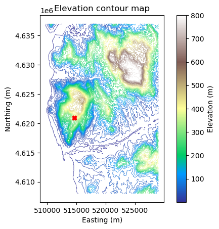
ax = wk.plot.elevation_map(elev_map, zorder=0)
wk.spatial.ds_to_gdf(bwc).plot(ax=ax, zorder=1, color="red", marker="X", markersize=40)
[7]:
<Axes: title={'center': 'Elevation contour map'}, xlabel='Easting (m)', ylabel='Northing (m)'>
[8]:
ax_lc = wk.plot.landcover_map(landcover_map, zorder=0)
wk.spatial.ds_to_gdf(bwc).plot(ax=ax_lc, zorder=1, color="black", marker="X", markersize=40)
[8]:
<Axes: xlabel='Easting (m)', ylabel='Northing (m)'>
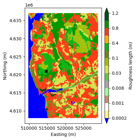
From the maps we can clearly observe the coast of the Atlantic ocean to the west as well as the river Limia which flows into the ocean. The geopandas dataframe also has a nice function called explore(), that opens the map in interactive window where you can zoom in on the features of the map and hover over areas.
[9]:
landcover_map.explore("z0")
[9]:
Output Locations#
Next up we will take a look at the site effects for the future turbine location. We need to tell pywasp what location we would like to calculate the site effects at. This is done by creating a xarray.Dataset with dimensions (west_east, south_north, and height) with coordinates values where we want to calculate the effects. Since this is a common need in PyWAsP, a convience function create_dataset has been created for this purpose.
We tell pywasp that the projection of west_east, south_north coordinates are in a UTM zone 29 by adding the attribute epsg giving it the integer number 32629.
[10]:
output_locs =  wk.spatial.create_point(
    west_east=np.array([514013.1]),
    south_north=np.array([4617763]),
    height=np.array([50]),
    crs=32629
)
print(output_locs)
<xarray.Dataset> Size: 33B
Dimensions:      (point: 1)
Coordinates:
    height       (point) int64 8B 50
    south_north  (point) int64 8B 4617763
    west_east    (point) float64 8B 5.14e+05
    crs          int8 1B 0
Dimensions without coordinates: point
Data variables:
    output       (point) float64 8B 0.0
Attributes:
    Conventions:  CF-1.8
    history:      2025-07-04T13:07:15+00:00:\twindkit==1.0.0\t"point")
Site effects#
Before generalizing the observed wind climate we read in earlier, we will take a look at the site effects at the mast location.
Let us first explore the roughness elements around the mast for each of 12 sectors. We can do this by using get_rou_rose method of topo_map, and pass in the location of the mast, note that roses are 2D so the height doesn’t matter in this case, and the number of sectors we would like to use. It requires a WAsP configuration object (pywasp.wasp.Config) that stores the parameters. We will simply use the default values.
PyWAsP will use the location information on the first object passed in (it must be a xr.Dataset), so we can use the bwc object to get the effects at the mast location.
[11]:
rou_rose, _ = topo_map.get_rou_rose(bwc, n_sectors=12)
wk.plot.roughness_rose(rou_rose)
Data type cannot be displayed: application/vnd.plotly.v1+json
The presence of the Atlantic ocean is clearly visible to the west, and we see that the rose corresponds well to what we would expect from the roughness elements we saw in the map.
To get the site effects we will use the get_site_effects method from our topo_map object.
get_site_effects expects the unique west_east and south_north values, the number of sectors, and the height above ground, and the configuration object.
pywasp note depending on the number of locations,
get_site_effectsmay take some time to complete
[12]:
site_effects = topo_map.get_site_effects(bwc, n_sectors=12)
print(site_effects)
print(site_effects.data_vars)
<xarray.Dataset> Size: 945B
Dimensions:              (point: 1, sector: 12)
Coordinates:
    height               (point) float64 8B 25.3
    crs                  int8 1B 0
    west_east            (point) float64 8B 5.147e+05
    south_north          (point) float64 8B 4.621e+06
    sector_ceil          (sector) float64 96B 15.0 45.0 75.0 ... 315.0 345.0
    sector_floor         (sector) float64 96B 345.0 15.0 45.0 ... 285.0 315.0
  * sector               (sector) float64 96B 0.0 30.0 60.0 ... 300.0 330.0
Dimensions without coordinates: point
Data variables: (12/15)
    z0meso               (sector, point) float32 48B 0.137 0.2776 ... 0.009736
    slfmeso              (sector, point) float32 48B 0.9432 1.0 ... 0.403 0.5834
    displ                (sector, point) float32 48B 0.0 0.0 0.0 ... 0.0 0.0 0.0
    flow_sep_height      (sector, point) float32 48B 0.0 0.0 0.0 ... 0.0 0.0 0.0
    user_def_speedups    (sector, point) float32 48B 1.0 1.0 1.0 ... 1.0 1.0 1.0
    orographic_speedups  (sector, point) float32 48B 1.156 1.206 ... 1.43 1.284
    ...                   ...
    orographic_turnings  (sector, point) float32 48B -2.929 6.098 ... -7.953
    obstacle_turnings    (sector, point) float32 48B 0.0 0.0 0.0 ... 0.0 0.0 0.0
    roughness_turnings   (sector, point) float32 48B 0.0 0.0 0.0 ... 0.0 0.0 0.0
    site_elev            (point) float32 4B 381.0
    rix                  (point) float32 4B 0.04571
    dirrix               (sector, point) float32 48B 0.001304 ... 0.06163
Attributes:
    Conventions:      CF-1.8
    history:          2025-07-04T13:07:08+00:00:\twindkit==1.0.0\tcreate_data...
    description:      SerraSantaluzia
    Package name:     windkit
    Package version:  1.0.0
    Creation date:    2025-07-04T13:07:17+00:00
    Object type:      Topographic effects
    author:           Bjarke Tobias Olsen
    author_email:     btol@dtu.dk
    institution:      DTU Wind
    title:            WAsP site effects
Data variables:
    z0meso               (sector, point) float32 48B 0.137 0.2776 ... 0.009736
    slfmeso              (sector, point) float32 48B 0.9432 1.0 ... 0.403 0.5834
    displ                (sector, point) float32 48B 0.0 0.0 0.0 ... 0.0 0.0 0.0
    flow_sep_height      (sector, point) float32 48B 0.0 0.0 0.0 ... 0.0 0.0 0.0
    user_def_speedups    (sector, point) float32 48B 1.0 1.0 1.0 ... 1.0 1.0 1.0
    orographic_speedups  (sector, point) float32 48B 1.156 1.206 ... 1.43 1.284
    obstacle_speedups    (sector, point) float32 48B 1.0 1.0 1.0 ... 1.0 1.0 1.0
    roughness_speedups   (sector, point) float32 48B 1.008 1.026 ... 0.891
    user_def_turnings    (sector, point) float32 48B 0.0 0.0 0.0 ... 0.0 0.0 0.0
    orographic_turnings  (sector, point) float32 48B -2.929 6.098 ... -7.953
    obstacle_turnings    (sector, point) float32 48B 0.0 0.0 0.0 ... 0.0 0.0 0.0
    roughness_turnings   (sector, point) float32 48B 0.0 0.0 0.0 ... 0.0 0.0 0.0
    site_elev            (point) float32 4B 381.0
    rix                  (point) float32 4B 0.04571
    dirrix               (sector, point) float32 48B 0.001304 ... 0.06163
The site effects dataset is made up of following variables:
z0meso: effective upstream roughness by sectorslfmeso: effective upstream sea-land-fraction by sectordispl: displacement height by sectoruser_def_speedups: user defined speed-ups (as factor)orographic_speedups: speed-ups due to orography (as factor)obstacle_speedups: obstacle induced speed-ups (as factor)roughness_speedups: speed-ups due to roughness changes (as factor)user_def_turnings: user defined wind turning (in degrees)orographic_turnings: wind turning due to orography (in degrees)obstacle_turnings: wind turning due to obstracels (in degrees)roughness_turnings: wind turning due to roughness changes (in degrees)elev: surface elevationrix: ruggedness indexdirrix: sector wise ruggedness index
The generalized wind climate calculation#
Now it is time to actually generalize our observed wind climate and then downscale it to our chosen turbine location. The generalized wind climate is a site-independent characterization of the wind climate for the entire Waspdale area. Generalization involves calculating the wind speed for predefined surface roughnesses and heights above ground. So the first thing we need to do is chose these roughness and height classes. Typically, the wind climate contains up to 5 standard heights and 5 standard roughness classes.
In a generalized wind climate data set the wind observations have been ‘cleaned’ with respect to the site-specific conditions. The data sets are site-independent and the wind distributions have been referenced to five standard roughness classes and five standard height above ground level.
[13]:
gen_roughnesses = np.array([0.0, 0.001, 0.03, 0.1, 0.4, 1.5])  # 5 standard roughness classes
gen_heights = np.array([10.0, 50.0, 100.0, 150.0, 200.0])  # 5 standard height classes
The generalization is done with the generalize function from pywasp’s wasp module. It takes the binned wind climate (bwc), our topographic map (topo_map), the roughness and height classes, and finally the configuration object (conf).
[14]:
gwc = pw.wasp.generalize(bwc, topo_map, gen_roughnesses=gen_roughnesses, gen_heights=gen_heights)
print(gwc)
<xarray.Dataset> Size: 5kB
Dimensions:        (point: 1, sector: 12, gen_height: 5, gen_roughness: 6)
Coordinates:
    height         (point) float64 8B 25.3
    south_north    (point) float64 8B 4.621e+06
    west_east      (point) float64 8B 5.147e+05
    crs            int8 1B 0
    sector_ceil    (sector) float64 96B 15.0 45.0 75.0 ... 285.0 315.0 345.0
    sector_floor   (sector) float64 96B 345.0 15.0 45.0 ... 255.0 285.0 315.0
  * sector         (sector) float64 96B 0.0 30.0 60.0 90.0 ... 270.0 300.0 330.0
  * gen_roughness  (gen_roughness) float64 48B 0.0 0.001 0.03 0.1 0.4 1.5
  * gen_height     (gen_height) float64 40B 10.0 50.0 100.0 150.0 200.0
Dimensions without coordinates: point
Data variables:
    A              (sector, gen_height, gen_roughness, point) float32 1kB 5.6...
    k              (sector, gen_height, gen_roughness, point) float32 1kB 1.7...
    wdfreq         (sector, gen_height, gen_roughness, point) float32 1kB 0.0...
    site_elev      (point) float32 4B 381.0
Attributes:
    Conventions:      CF-1.8
    history:          2025-07-04T13:07:08+00:00:\twindkit==1.0.0\tcreate_data...
    description:      SerraSantaluzia
    Package name:     windkit
    Package version:  1.0.0
    Creation date:    2025-07-04T13:07:18+00:00
    Object type:      Geostrophic Wind Climate
    author:           Bjarke Tobias Olsen
    author_email:     btol@dtu.dk
    institution:      DTU Wind
    title:            Generalized wind climate
The generalized wind climate contains weibull parameters (A and k) for each location, sector, and height and roughness class.
Estimating wind power#
Now that we have calculated a generalised wind climate (GWC) with site-independent wind climate data, we can apply those data to prospect turbine sites. PyWAsP can adjust the data for the situation found at the turbine site and produce a prediction of the wind climate for the site itself.
The pywasp.wasp module provides two ways of doing this: downscale and get_wasp_down. The latter assumes site effects that have already been calculated, while the first one will start by calculating them. Since we have already calculated the site effects, we will use get_wasp_down. The function requires passing a genwc_interp method. Two choices are available: 'nearest' and 'natural'. This is important when several generalized wind climates are present and will tell
pywasp how to interpolate them to the location. Since just one wind climate is present in this study, the same generalized wind climate will be used everywhere.
To estimate the the power production for a turbine positioned at the site we need to add a turbine wind turbine generator object that holds the power curve and other information about the characteristics of the turbine. We will read a Wind Turbine Generator dataset using pw.io.read_wtg. The turbine used here is the Bonus 1 MW wind turbine.
[15]:
wtg = wk.read_wtg("./data/Bonus_1_MW.wtg")
print(wtg)
<xarray.Dataset> Size: 704B
Dimensions:                        (mode: 1, wind_speed: 22)
Coordinates:
  * wind_speed                     (wind_speed) float64 176B 4.0 5.0 ... 25.0
  * mode                           (mode) int64 8B 0
Data variables:
    power_output                   (mode, wind_speed) float64 176B 2.41e+04 ....
    thrust_coefficient             (mode, wind_speed) float64 176B 0.915 ... ...
    air_density                    (mode) float64 8B 1.225
    stationary_thrust_coefficient  (mode) float64 8B 0.161
    wind_speed_cutin               (mode) float64 8B 4.0
    wind_speed_cutout              (mode) float64 8B 25.0
    rated_power                    (mode) float64 8B 1e+06
    name                           <U10 40B 'Bonus 1 MW'
    manufacturer                   <U16 64B 'Bonus Energy A/S'
    rotor_diameter                 float64 8B 54.2
    hub_height                     float64 8B 50.0
    regulation_type                int64 8B 2
Attributes:
    Conventions:      CF-1.8
    Package name:     windkit
    Package version:  1.0.0
    Creation date:    2025-07-04T13:07:19+00:00
    author:           Bjarke Tobias Olsen
    author_email:     btol@dtu.dk
    institution:      DTU Wind
We can see that the dataset holds the information about the WTG, including:
Power and thrust coefficient curves for varying wind speeds
Wind speed cutin and cutout
Rated power
Rotor diameter
Hub height
The WTG can have different modes with different values for different air density situations for example. This WTG has 1 mode for the standard air density of 1.225 kg / m^3.
Nonetheless, the WTG power curve will, by default, get corrected for the site-specific air density when estiamting the AEP. A higher than 1.225 kg / m^3 air density will result in an upwards shift of the power curve, while a lower air density will result in a downwards shift.
To plot the power and thrust coefficient curves we can use the plotting function plot_wtg_curves from PyWAsP:
[16]:
wk.plot.power_ct_curves(wtg)
Data type cannot be displayed: application/vnd.plotly.v1+json
Now that we have the turbine data we can combine it with a location in our map to predict the power. We will add the location and hub height of our turbine to xr.Dataset we can create by using the built-in create_dataset in PyWAsP:
[17]:
x, y, hub_height = 514325, 4622375, 50.0
turbine_loc =  wk.spatial.create_point([x], [y], [hub_height], crs="EPSG:32629")
Lets plot the turbine location on the elevation map to see where it’s located.
[18]:
ax = wk.plot.elevation_map(elev_map, zorder=0)
wk.spatial.ds_to_gdf(bwc).plot(ax=ax, color="red", marker="X", markersize=40, zorder=1)
wk.spatial.ds_to_gdf(turbine_loc).plot(ax=ax, color="black", marker="X", markersize=40, zorder=2)
[18]:
<Axes: title={'center': 'Elevation contour map'}, xlabel='Easting (m)', ylabel='Northing (m)'>
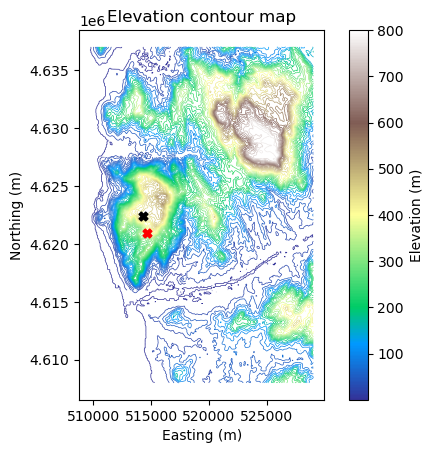
We can see that the wind turbine is located on a local peak on the hill to the west in the map near the coastline. Next up, we will calculate the power production for the turbine. To do this, we will first calculate the wind climate at the location of the turbine hub height using PyWAsP’s downscale function which takes in a generalized wind climate, the topography data, the turbine position(s) and hub height(s), the wasp configuration, and we also add the genwc_interp=nearest"
keyword to tell PyWAsP we want it to use the nearest GWC to each turbine (in this case its always the same, since we only have one GWC).
[19]:
pwc = pw.wasp.downscale(gwc, topo_map, turbine_loc, interp_method="nearest")
print(pwc)
<xarray.Dataset> Size: 473B
Dimensions:        (point: 1, sector: 12)
Coordinates:
    height         (point) float64 8B 50.0
    south_north    (point) int64 8B 4622375
    west_east      (point) int64 8B 514325
    crs            int8 1B 0
    sector_ceil    (sector) float64 96B 15.0 45.0 75.0 ... 285.0 315.0 345.0
    sector_floor   (sector) float64 96B 345.0 15.0 45.0 ... 255.0 285.0 315.0
  * sector         (sector) float64 96B 0.0 30.0 60.0 90.0 ... 270.0 300.0 330.0
Dimensions without coordinates: point
Data variables:
    A              (sector, point) float32 48B 7.041 6.572 6.188 ... 7.326 7.172
    k              (sector, point) float32 48B 2.041 2.385 2.498 ... 2.248 2.092
    wdfreq         (sector, point) float32 48B 0.063 0.0392 ... 0.09475 0.08239
    site_elev      (point) float32 4B 460.0
    air_density    (point) float32 4B 1.163
    wspd           (point) float32 4B 6.998
    power_density  (point) float32 4B 344.5
Attributes:
    Conventions:      CF-1.8
    history:          2025-07-04T13:07:19+00:00:\twindkit==1.0.0\t"point")\n2...
    title:            WAsP site effects
    Package name:     windkit
    Package version:  1.0.0
    Creation date:    2025-07-04T13:07:21+00:00
    Object type:      Met fields
    author:           Bjarke Tobias Olsen
    author_email:     btol@dtu.dk
    institution:      DTU Wind
We can now combine the predicted wind climate with the wind turbine generator to get the annual power production.
[20]:
aep = pw.gross_aep(pwc, wtg)
print(aep)
<xarray.Dataset> Size: 365B
Dimensions:           (point: 1, sector: 12)
Coordinates:
    height            (point) float64 8B 50.0
    south_north       (point) int64 8B 4622375
    west_east         (point) int64 8B 514325
    crs               int8 1B 0
    sector_ceil       (sector) float64 96B 15.0 45.0 75.0 ... 285.0 315.0 345.0
    sector_floor      (sector) float64 96B 345.0 15.0 45.0 ... 255.0 285.0 315.0
  * sector            (sector) float64 96B 0.0 30.0 60.0 ... 270.0 300.0 330.0
Dimensions without coordinates: point
Data variables:
    gross_aep         (point) float32 4B 2.466
    gross_aep_sector  (point, sector) float32 48B 0.1235 0.06057 ... 0.1672
Attributes:
    Conventions:      CF-1.8
    history:          2025-07-04T13:07:19+00:00:\twindkit==1.0.0\t"point")\n2...
    title:            WAsP site effects
    Package name:     windkit
    Package version:  1.0.0
    Creation date:    2025-07-04T13:07:21+00:00
    Object type:      Anual Energy Production
    author:           Bjarke Tobias Olsen
    author_email:     btol@dtu.dk
    institution:      DTU Wind
As we can see, the predicted power production for the turbine at the site is 2.6 GWh/y
Estimating wind farm production#
Now that we have estimated the power for a single turbine, we can look at the power production for a whole wind farm. The workflow is indentical to the one we just used for a single turbine. We have predefined some turbine positions in the data/turbine_positions.csv file, so lets create the location dataset and plot the turbines on our map.
[21]:
wtg_locs = pd.read_csv('./data/turbine_positions.csv')

wind_turbines = wk.create_wind_turbines_from_arrays(
    west_east=wtg_locs["Easting"].values,
    south_north=wtg_locs["Northing"].values,
    height=wtg_locs["Hub height"].values,
    wtg_keys=["Bonus_1_MW"]*wtg_locs.shape[0],
    crs="EPSG:32629"
)

wind_turbines
[21]:
<xarray.Dataset> Size: 1kB
Dimensions:      (point: 15)
Coordinates:
    height       (point) int64 120B 50 50 50 50 50 50 50 50 50 50 50 50 50 50 50
    south_north  (point) int64 120B 4622313 4622199 4622336 ... 4624252 4624142
    west_east    (point) int64 120B 513914 514161 514425 ... 516060 516295
    crs          int8 1B 0
    turbine_id   (point) int64 120B 0 1 2 3 4 5 6 7 8 9 10 11 12 13 14
    group_id     (point) float64 120B 0.0 0.0 0.0 0.0 0.0 ... 0.0 0.0 0.0 0.0
    wtg_key      (point) <U10 600B 'Bonus_1_MW' 'Bonus_1_MW' ... 'Bonus_1_MW'
Dimensions without coordinates: point
Data variables:
    *empty*
Attributes:
    Conventions:  CF-1.8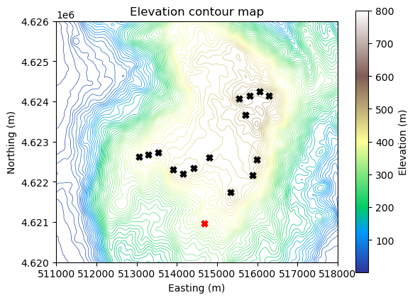
history: 2025-07-04T13:07:21+00:00:\twindkit==1.0.0\tcreate_dataset(We can see that the turbines are mostly on the (locally) highest points in the terrain.
[22]:
ax = wk.plot.elevation_map(elev_map, zorder=0)
wk.spatial.ds_to_gdf(bwc).plot(ax=ax, color="red", marker="X", markersize=40, zorder=1)
wk.spatial.ds_to_gdf(wind_turbines).plot(ax=ax, color="black", marker="X", markersize=40, zorder=1)
ax.set(xlim=(511000, 518000), ylim=(4620000, 4626000))
[22]:
[(511000.0, 518000.0), (4620000.0, 4626000.0)]
To calculate the predicted wind climates at the 15 positions (at 50 m AGL) we will again use the downscale function.
[23]:
pwc = pw.wasp.downscale(gwc, topo_map, wind_turbines, interp_method="nearest")
Now we can calculate the AEP
[24]:
aep_nowake = pw.gross_aep(pwc, wtg)

aep_nowake = aep_nowake["gross_aep"]
print(aep_nowake)
print(aep_nowake.sum())
<xarray.DataArray 'gross_aep' (point: 15)> Size: 60B
array([2.8252254, 2.687702 , 2.4737535, 2.5607786, 2.727687 , 2.807531 ,
       2.6752436, 2.969323 , 3.060742 , 2.307256 , 2.6991627, 2.9334679,
       2.889413 , 3.0800772, 3.2932563], dtype=float32)
Coordinates:
    height       (point) int64 120B 50 50 50 50 50 50 50 50 50 50 50 50 50 50 50
    south_north  (point) int64 120B 4622313 4622199 4622336 ... 4624252 4624142
    west_east    (point) int64 120B 513914 514161 514425 ... 516060 516295
    crs          int8 1B 0
    turbine_id   (point) int64 120B 0 1 2 3 4 5 6 7 8 9 10 11 12 13 14
    group_id     (point) float64 120B 0.0 0.0 0.0 0.0 0.0 ... 0.0 0.0 0.0 0.0
    wtg_key      (point) <U10 600B 'Bonus_1_MW' 'Bonus_1_MW' ... 'Bonus_1_MW'
Dimensions without coordinates: point
Attributes:
    description:    Gross annual energy production, without considering wake ...
    long_name:      Gross annual energy production
    standard_name:  gross_aep
    units:          GWh
    grid_mapping:   crs
<xarray.DataArray 'gross_aep' ()> Size: 4B
array(41.99062, dtype=float32)
Coordinates:
    crs      int8 1B 0
We get back an AEP for each turbine. In total we estimate that our wind farm produces about 42 Gwh annually, without taking wake effects and other losses into account.
Notice that if we would not be correcting for air density, the 1.225 kg/m^3 reference power curve would be used, achieving a virtually less accurate result of 43.7 GWh annually. This can be checked by setting the air_density_correction = "none".
Lets now use wake effects in the AEP calculations to see how much these affect our annual power production. PyWAsP uses PyWake internally to take wake effects into account.
Several wake models can be used, but we will use the wake model that corresponds to the wake model found in the offical WAsP GUI software for Windows, called “PARK2” in PyWAsP.
[25]:
aep_park2 = pw.potential_aep(
    pwc,
    wtg,
    wind_farm_model="PARK2_onshore",
    turbulence_intensity=0.0
)

aep_park2 = aep_park2["potential_aep"]
print(aep_park2)
print(aep_park2.sum())
<xarray.DataArray 'potential_aep' (point: 15)> Size: 120B
array([2.7278782 , 2.59931447, 2.36980802, 2.45435784, 2.62128109,
       2.76544897, 2.64794008, 2.92111536, 3.00184219, 2.23764838,
       2.64323762, 2.84922645, 2.74544182, 2.91545043, 3.17742836])
Coordinates:
    height       (point) int64 120B 50 50 50 50 50 50 50 50 50 50 50 50 50 50 50
    south_north  (point) int64 120B 4622313 4622199 4622336 ... 4624252 4624142
    west_east    (point) int64 120B 513914 514161 514425 ... 516060 516295
    crs          int8 1B 0
    turbine_id   (point) int64 120B 0 1 2 3 4 5 6 7 8 9 10 11 12 13 14
    group_id     (point) float64 120B 0.0 0.0 0.0 0.0 0.0 ... 0.0 0.0 0.0 0.0
    wtg_key      (point) <U10 600B 'Bonus_1_MW' 'Bonus_1_MW' ... 'Bonus_1_MW'
    mode         int64 8B 0
  * point        (point) int64 120B 0 1 2 3 4 5 6 7 8 9 10 11 12 13 14
Attributes:
    description:    Potential annual energy production, considering wake effe...
    long_name:      Potential annual energy production
    standard_name:  potential_aep
    units:          GWh
    grid_mapping:   crs
<xarray.DataArray 'potential_aep' ()> Size: 8B
array(40.67741931)
Coordinates:
    crs      int8 1B 0
    mode     int64 8B 0
We can see that wake effects causes a reduction of the AEP from 42 to 40.7 GWh/y (a 3.3 % reduction).
Let us visaulize the turbine-by-turbine AEP and reduction by wake effects.
[26]:
fig, axes = plt.subplots(1, 2, figsize=(15, 5))
aep_nowake.plot(ax=axes[0], marker="o", color="blue", label=f"No wakes: {aep_nowake.sum().values:.1f} [GWh]")
aep_park2.plot(ax=axes[0], marker="*", markersize=8, label=f"Wakes: {aep_park2.sum().values:.1f} [GWh]", color="green")

(aep_park2 / aep_nowake).plot(ax=axes[1], marker="s", color="C1")

# Add grid to both plots
axes[0].grid(True, linestyle="--", alpha=0.7)
axes[1].grid(True, linestyle="--", alpha=0.7)

# Add subtitles to each plot
axes[0].set_title("Gross vs Potential AEP", fontsize=14)
axes[1].set_title("Ratio of Potential to Gross AEP", fontsize=14)

# Set x-axis and y-axis labels
axes[0].set(xlabel="Wind Turbine id", ylabel="AEP [GWh]", ylim=(2, 4))
axes[1].set(xlabel="Wind Turbine id", ylabel=r"AEP / AEP$_\mathrm{no wakes}$")

axes[0].legend(frameon=False, title="Wake model")

plt.show()
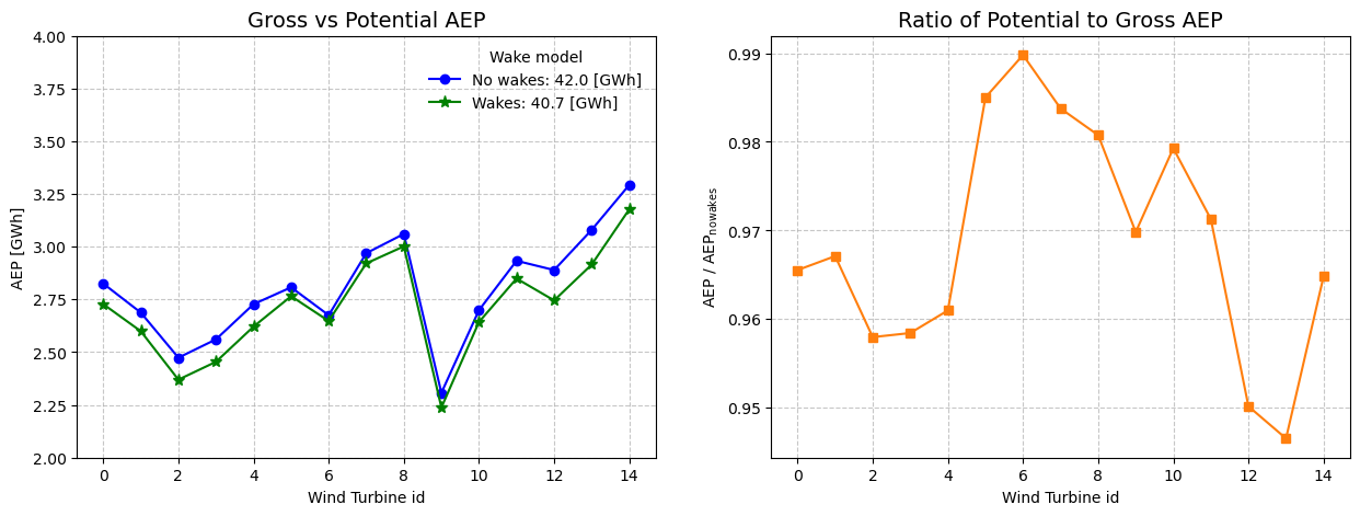
The First plot shows the AEP for each turbine. It varies alot from turbine to turbine due to the differences in the local wind climate.
The second plot shows the relative decrease in AEP due to wake effects. We can see that turbine at index 12 and 13 (Index starts at 0) are affected (relatively) most by wake effects, with their AEP reduced by about 5%.
[27]:
output_grid = wk.spatial.create_cuboid(
    west_east=np.linspace(511700.0, 517700.0, 41),
    south_north=np.linspace(4619500.0, 4625500.0, 41),
    height=[50.0],
    crs="EPSG:32629",
)

pwc_grid = pw.wasp.downscale(gwc, topo_map, output_grid)
pwc_grid
[27]:
<xarray.Dataset> Size: 270kB
Dimensions:        (sector: 12, height: 1, south_north: 41, west_east: 41)
Coordinates:
    crs            int8 1B 0
    sector_ceil    (sector) float64 96B 15.0 45.0 75.0 ... 285.0 315.0 345.0
    sector_floor   (sector) float64 96B 345.0 15.0 45.0 ... 255.0 285.0 315.0
  * height         (height) float64 8B 50.0
  * south_north    (south_north) float64 328B 4.62e+06 4.62e+06 ... 4.626e+06
  * west_east      (west_east) float64 328B 5.117e+05 5.118e+05 ... 5.177e+05
  * sector         (sector) float64 96B 0.0 30.0 60.0 90.0 ... 270.0 300.0 330.0
Data variables:
    A              (sector, height, south_north, west_east) float32 81kB 5.16...
    k              (sector, height, south_north, west_east) float32 81kB 1.98...
    wdfreq         (sector, height, south_north, west_east) float32 81kB 0.06...
    site_elev      (south_north, west_east) float32 7kB 15.3 22.06 ... 199.8
    air_density    (height, south_north, west_east) float32 7kB 1.216 ... 1.194
    wspd           (height, south_north, west_east) float32 7kB 5.545 ... 4.86
    power_density  (height, south_north, west_east) float32 7kB 200.1 ... 121.8
Attributes:
    Conventions:      CF-1.8
    history:          2025-07-04T13:07:45+00:00:\twindkit==1.0.0\t"cuboid")\n...
    Package name:     windkit
    Package version:  1.0.0
    Creation date:    2025-07-04T13:07:50+00:00
    Object type:      Met fields
    author:           Bjarke Tobias Olsen
    author_email:     btol@dtu.dk
    institution:      DTU Wind
title: WAsP site effects[28]:
flow_map = pw.wind_farm_flow_map(
    pwc_grid,
    wtg,
    wind_turbines,
    output_grid,
    wind_farm_model="PARK2_onshore",
    turbulence_intensity=0.0,
    n_subsector=5,
)
print(flow_map)
<xarray.Dataset> Size: 1MB
Dimensions:                          (sector: 12, height: 1, south_north: 41,
                                      west_east: 41)
Coordinates:
    crs                              int8 1B 0
    mode                             int64 8B 0
  * sector                           (sector) float64 96B 0.0 30.0 ... 330.0
  * height                           (height) float64 8B 50.0
  * south_north                      (south_north) float64 328B 4.62e+06 ... ...
  * west_east                        (west_east) float64 328B 5.117e+05 ... 5...
Data variables: (12/15)
    potential_aep_sector             (sector, height, south_north, west_east) float64 161kB ...
    gross_aep_sector                 (sector, height, south_north, west_east) float64 161kB ...
    potential_aep_deficit_sector     (sector, height, south_north, west_east) float64 161kB ...
    wspd_sector                      (sector, height, south_north, west_east) float64 161kB ...
    wspd_eff_sector                  (sector, height, south_north, west_east) float64 161kB ...
    wspd_deficit_sector              (sector, height, south_north, west_east) float64 161kB ...
    ...                               ...
    gross_aep                        (height, south_north, west_east) float64 13kB ...
    potential_aep_deficit            (height, south_north, west_east) float64 13kB ...
    wspd                             (height, south_north, west_east) float64 13kB ...
    wspd_eff                         (height, south_north, west_east) float64 13kB ...
    wspd_deficit                     (height, south_north, west_east) float64 13kB ...
    turbulence_intensity_eff         (height, south_north, west_east) float64 13kB ...
Attributes:
    Conventions:      CF-1.8
    history:          2025-07-04T13:07:45+00:00:\twindkit==1.0.0\t"cuboid")\n...
    Package name:     windkit
    Package version:  1.0.0
    Creation date:    2025-07-04T13:08:02+00:00
    Object type:      Wind Farm Flow Map
    author:           Bjarke Tobias Olsen
    author_email:     btol@dtu.dk
    institution:      DTU Wind
    title:            WAsP site effects
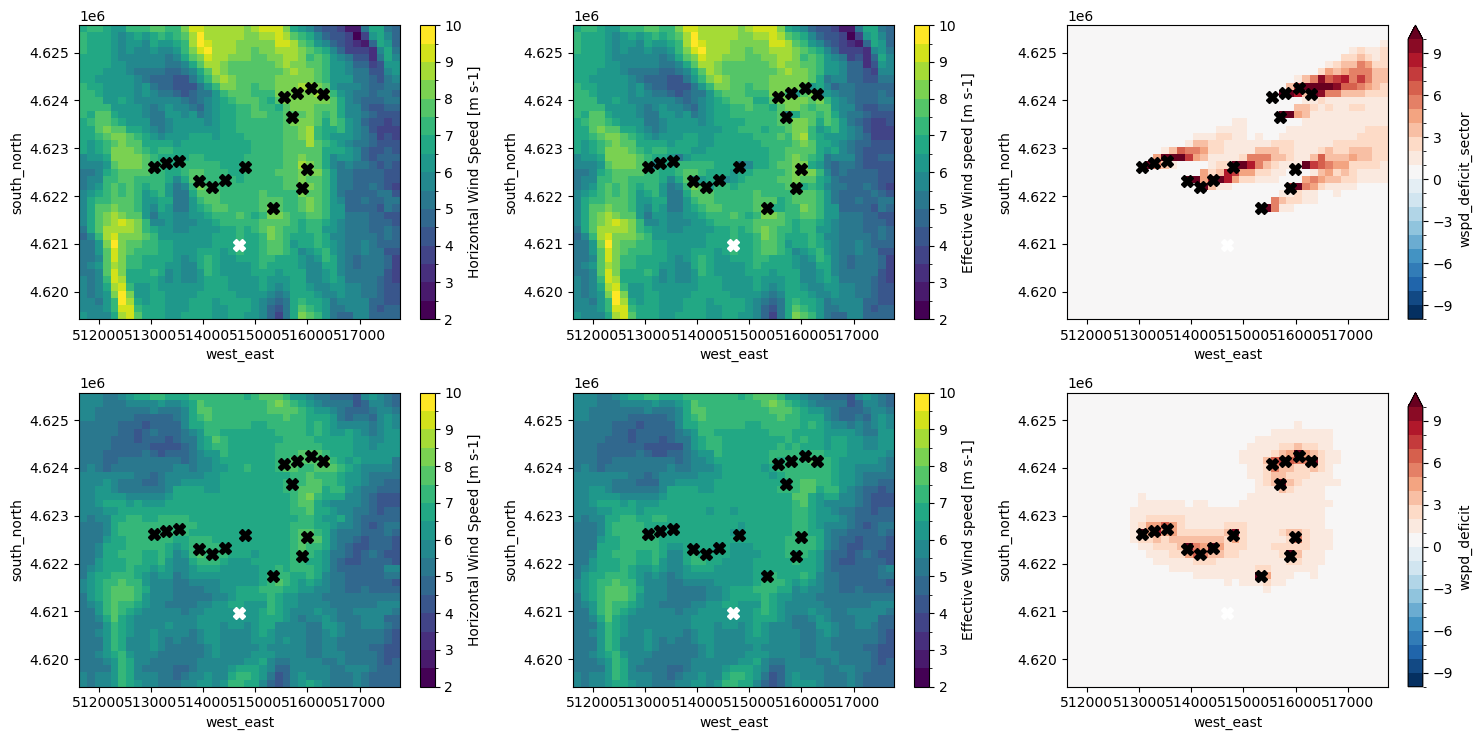
[29]:
fig, axes = plt.subplots(2, 3, figsize=(15, 7.5))
flow_map["wspd_sector"].sel(sector=240).plot(ax=axes[0, 0], levels=np.linspace(2.0, 10.0, 17))
flow_map["wspd_eff_sector"].sel(sector=240).plot(ax=axes[0, 1], levels=np.linspace(2.0, 10.0, 17))
(100.0 * flow_map["wspd_deficit_sector"]).sel(sector=240).plot(ax=axes[0, 2], levels=np.linspace(-10.0, 10.0, 21))
flow_map["wspd"].plot(ax=axes[1, 0], levels=np.linspace(2.0, 10.0, 17))
flow_map["wspd_eff"].plot(ax=axes[1, 1], levels=np.linspace(2.0, 10.0, 17))
(100.0 * flow_map["wspd_deficit"]).plot(ax=axes[1, 2], levels=np.linspace(-10.0, 10.0, 21))
for ax in axes.flat:
    ax.plot(wind_turbines.west_east, wind_turbines.south_north, ls="none", marker="X", markersize=8, color="black")
    ax.plot(bwc.west_east, bwc.south_north, marker="X", color="white", markersize=8)
    ax.set(title="")
plt.tight_layout()
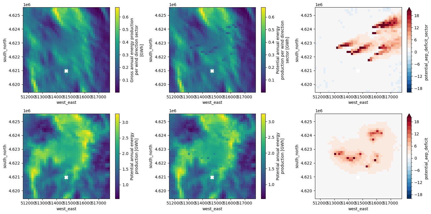
[30]:
fig, axes = plt.subplots(2, 3, figsize=(15, 7.5))
flow_map["gross_aep_sector"].sel(sector=240).plot(ax=axes[0, 0])
flow_map["potential_aep_sector"].sel(sector=240).plot(ax=axes[0, 1])
(100.0 * flow_map["potential_aep_deficit_sector"]).sel(sector=240).plot(ax=axes[0, 2], levels=np.linspace(-20.0, 20.0, 21))
flow_map["gross_aep"].plot(ax=axes[1, 0])
flow_map["potential_aep"].plot(ax=axes[1, 1])
(100.0 * flow_map["potential_aep_deficit"]).plot(ax=axes[1, 2], levels=np.linspace(-20.0, 20.0, 21))
for ax in axes.flat:
    ax.plot(output_locs.west_east, output_locs.south_north, ls="none", marker="X", markersize=8, color="black")
    ax.plot(bwc.west_east, bwc.south_north, marker="X", color="white", markersize=8)
    ax.set(title="")
plt.tight_layout()