PyWAsP: From observed wind climate to resource map#
Introduction#
This is an interactive tutorial that will introduce you to the basic WAsP workflow using PyWAsP.
After completing this tutorial you will be familiar with basic pywasp functionality, including:
opening and inspecting wind climate files;
opening map files and inspecting terrain data;
calculating and inspecting terrain-induced effects on the wind at various sites;
creating a generalized wind climate from the observed wind climate;
creating a resource map by “downscaling” the generalized wind climate.
As you work your way through the notebook, make sure to run the python code in each cell, in the order that the cells appear. You run the code by clicking on the cell (outlines around the cell should appear) and pressing <shift> + <enter> on the keyboard.
notebook note if something looks wrong, or when errors occur, it can be helpful to restart the python kernel via the kernel tab in the top
Import packages#
Usually the first step when writing (or using) a python program is to import the standard (external) packages we will need. For the analysis in this tutorial we will import numpy, matplotlib, xarray, windkit and pywasp itself.
numpyis python’s main numerical array package https://www.numpy.org/matplotlibis python’s main plotting package https://matplotlib.org/pywaspdocummentation is found at http://docs.wasp.dk/windkitdocumentation is found at http://docs.wasp.dk/windkit
We will also make references to
xarrayis a powerful high level package for labelled multi-dimensional arrays http://xarray.pydata.org
[1]:
import warnings

import numpy as np
import matplotlib.pyplot as plt

import windkit as wk
import pywasp as pw

warnings.filterwarnings('ignore')  # We will ignore warnings to avoid cluttering the notebook
It is common to make a short alias of a package when importing it, using the syntax import [package] as [short alias for package]; for example you can see import pywasp as pw above. The functions and classes of imported packages must be accessed through explicitly typing the package name or alias; e.g., np.cos(3.14) will use the cosine function from numpy.
Observed wind climate#
Now we will import our (observed) binned wind climate from the Høvsøre mast. The data is stored in hovsore.tab in the data folder. It represents the observed wind climate for the period 2007-2015 at 100 m above ground level.
pywasp note
pywaspincludes functionality to both read and write wind climate files in many data formats, including ascii (.tab), xml (.owc), and netCDF (.nc).
The geospatial coordinate in the file is in the European grid projection (EPSG:3035), which is the recommended projection for high-resolution studies in Europe. We will tell pywasp this by explicitly passing a keyword argument srs="EPSG:3035" to the open_bwc call.
[2]:
bwc = wk.read_bwc('data/hovsore.tab', crs="EPSG:3035")
print(bwc)
<xarray.Dataset> Size: 4kB
Dimensions:       (point: 1, sector: 12, wsbin: 30)
Coordinates:
    height        (point) float64 8B 100.0
    south_north   (point) float64 8B 3.706e+06
    west_east     (point) float64 8B 4.207e+06
    crs           int8 1B 0
    wsceil        (wsbin) float64 240B 1.0 2.0 3.0 4.0 ... 27.0 28.0 29.0 30.0
    wsfloor       (wsbin) float64 240B 0.0 1.0 2.0 3.0 ... 26.0 27.0 28.0 29.0
    sector_ceil   (sector) float64 96B 15.0 45.0 75.0 ... 285.0 315.0 345.0
    sector_floor  (sector) float64 96B 345.0 15.0 45.0 ... 255.0 285.0 315.0
  * wsbin         (wsbin) float64 240B 0.5 1.5 2.5 3.5 ... 26.5 27.5 28.5 29.5
  * sector        (sector) float64 96B 0.0 30.0 60.0 90.0 ... 270.0 300.0 330.0
Dimensions without coordinates: point
Data variables:
    wdfreq        (sector, point) float64 96B 0.02869 0.04459 ... 0.09727 0.0156
    wsfreq        (wsbin, sector, point) float64 3kB 0.01167 0.01544 ... 0.0 0.0
Attributes:
    Conventions:      CF-1.8
    history:          2025-07-04T13:11:55+00:00:\twindkit==1.0.0\tcreate_data...
    description:      Høvsøre observed wind climate EPSG:3035
    Package name:     windkit
    Package version:  1.0.0
    Creation date:    2025-07-04T13:11:55+00:00
    Object type:      Binned Wind Climate
    author:           Bjarke Tobias Olsen
    author_email:     btol@dtu.dk
    institution:      DTU Wind
Notice that the bwc object is of type <xarray.Dataset> and that it contains four kinds of data:
Dimensions: core named dimensions
Coordinates: coordinate values along dimensions
Data variables: named arrays with data along 0-N named dimensions
Attributes: additional meta data attached to the dataset
xarray note the primitive datatype and dimensions of each variable are also shown, along with a small sample of the data.
wsfreqis a four-dimensionalfloat64(double precision) variable along dimensions(wsbin, sector, height, point)
Xarray datasets wrap numpy arrays, annotating them with human-readable dimensions and coordinates, and allowing for easy subsetting, data manipulation, and plotting of the underlying data. An xarray.Dataset object is a collection of data variables, while each varible itself has type xarray.DataArray.
xarray note Use the
.valuesobject attribute to access the underlying numpy array
Beyond the wind speed and wind direction distributions, the wind climate contains information about the height of the measurements (height) and the geospatial location (west_east and south_north), which in this case hold the location information in the projected coordinates of the EPSG:3035 projection.
In the cell below, we will store the location of the Høvsøre mast in variables loc_x and loc_y for later use.
[3]:
loc_x = bwc['west_east'].item()
loc_y = bwc['south_north'].item()
The next step is to plot the wind rose and wind speed distributions in the binned wind climate. For convinience a plotting function plot_bwc has been implemented in pywasp_tutorial that will do this.
notebook note: you can view the documentation for a function in jupyter notebooks by placing a
?in front of the function, and you can get the entire function by using??.
[4]:
wk.plot.histogram_lines(bwc)
Data type cannot be displayed: application/vnd.plotly.v1+json
As expected for Denmark, the prevailing wind directions at Høvsøre are westerly; the wind sector with the greatest relative wind speeds is the sector centered on 300 degrees, and the lowest relative wind speeds comes from due north (though they are quite rare).
Topography data#
Now that we have inspected the wind climate, the next step is to load and inspect the terrain elevation data.
Terrain data (SRTM)#
For this tutorial we have provided SRTM elevation data near Høvsøre in a geoTIFF file, elev.tif. We will use pywasp to open this dataset with the read_rastermap command, telling pywasp that we are reading in an “elevation” raster type.
[5]:
elev = wk.read_elevation_map('data/elev.tif', map_type='elevation')
print(elev)
<xarray.DataArray 'elevation' (south_north: 800, west_east: 800)> Size: 5MB
[640000 values with dtype=float64]
Coordinates:
  * west_east    (west_east) float64 6kB 7.818 7.818 7.819 ... 8.482 8.483 8.483
  * south_north  (south_north) float64 6kB 56.11 56.11 56.11 ... 56.77 56.77
    crs          int64 8B 0
Attributes:
    description:    height above sea level of a point on the surface of an or...
    long_name:      Terrain Elevation
    standard_name:  ground_level_altitude
    units:          m
    grid_mapping:   crs
    history:        2025-07-04T13:11:56+00:00:\twindkit==1.0.0\t**kwargs)
Notice that while the bwc object was a collection of variables (<xarray.Dataset>), elev is a single data variable of type xarray.DataArray.
The elevation data is provided as a raster (i.e. not vector data), defined by {latitude, longitude} coordinates, in this case following the commonly-used WGS84 (World Geodetic System 1984) projection (EPSG:4326).
To transform our elevation data into the local projection (EPSG:3035), several approaches can be used in pywasp. Here we will re-project the data onto a new raster via interpolation using the warp function from pywasp.spatial. Because the re-projected raster contains missing data along the edges, the clip function is subsequently used to trim the raster to a smaller area containing no missing values.
[6]:
elev = wk.spatial.warp(elev, to_crs='EPSG:3035')  # Interpolate to local raster projection EPSG:3035
bounds = (4187500, 3686000, 4226500, 3725000)  # Bounds to trim to: specify box corners x_SW, y_SW, x_NE, y_NE
elev = wk.spatial.clip(elev, bounds)  # Trim data
print(elev)
<xarray.DataArray 'elevation' (south_north: 520, west_east: 520)> Size: 2MB
array([[ 0.,  0.,  0., ...,  0.,  0.,  0.],
       [ 0.,  0.,  0., ...,  0.,  0.,  0.],
       [ 0.,  0.,  0., ...,  0.,  0.,  0.],
       ...,
       [ 0.,  0.,  0., ..., 28., 27., 22.],
       [ 0.,  0.,  0., ..., 29., 27., 22.],
       [ 0.,  0.,  0., ..., 29., 27., 22.]], shape=(520, 520))
Coordinates:
    crs          int8 1B 0
  * south_north  (south_north) float64 4kB 3.725e+06 3.725e+06 ... 3.686e+06
  * west_east    (west_east) float64 4kB 4.188e+06 4.188e+06 ... 4.226e+06
Attributes:
    description:    height above sea level of a point on the surface of an or...
    long_name:      Terrain Elevation
    standard_name:  ground_level_altitude
    units:          m
    grid_mapping:   crs
    history:        2025-07-04T13:11:56+00:00:\twindkit==1.0.0\t**kwargs)
Let’s visualize the elevation data. To plot it on a map, we will use the plot method built into xarray.DataArray. We will use the terrain colormap, bound to values between -11 and 50, and plot it on a canvas 14x10 inches large.
xarray note
xarray.DataArray.plotwraps matplotlib functions with sensible defaults, which makes it easy to inspect the data “on the go”
To highlight the location of the mast, we use the matplotlib plot function, and tell it to plot a red dot (using the syntax or) of size 16.
To zoom in near the mast, extending 18 kilometers in each direction, we use matplotlib’s xlim and ylim functions.
[7]:
# Plot the elevation
elev.plot(x='west_east',
          y='south_north',
          cmap='terrain',
          vmin=-11,
          vmax=50,
          figsize=(14, 10))

# Add the Høvsøre mast location to the plot
plt.plot(loc_x, loc_y, 'or', ms=16)

# Define the plot extent
plt_extent = 18000.0

# Set the plot extent
plt.xlim([loc_x - plt_extent, loc_x + plt_extent])
plt.ylim([loc_y - plt_extent, loc_y + plt_extent]);
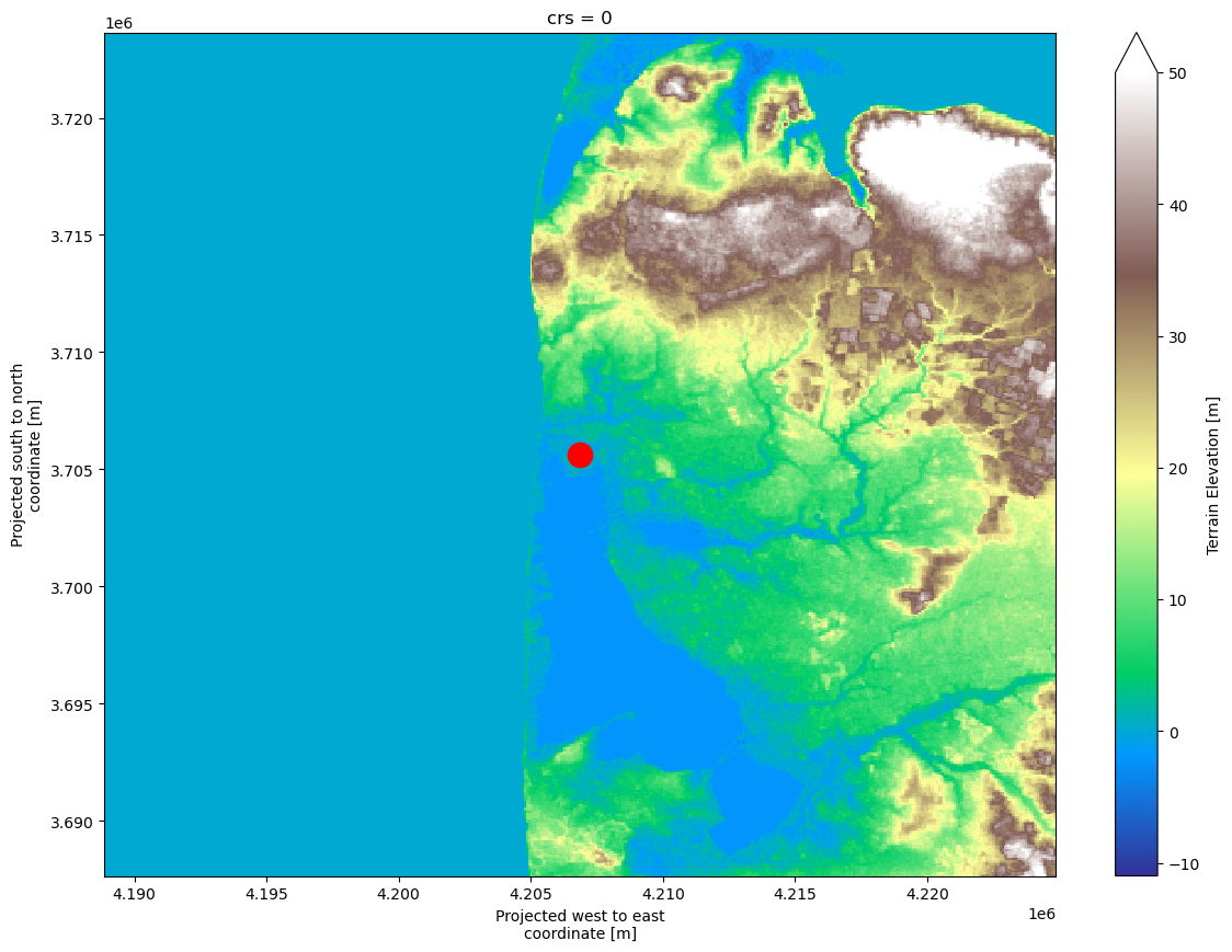
It is no surprise that Denmark is quite flat. But above, we can clearly see the coastline of Jutland stretching in the north-south direction.
Roughness data (CORINE LandCover)#
Next up is surface roughness. Here we start from a map of roughness lengths that was created based on the CORINE 2018 landcover dataset, using a “lookup table” which assigns particular lengths to each landcover type. The roughness map is provided as a GeoTiff file rough.tif; this is a common format in the GIS community. Conviniently, the CORINE dataset uses the European grid projection.
Even though this data is saved as a file of roughness values, when it is read into PyWAsP it is converted to a landcover map with a corresponding landcover lookup table. This is done to allow for easy manipulation of the different roughness values without having to manipulate the map itself. It also opens up for the possibility to include displacement heights and other relevant parameters, which will be explored more in Tutorial 3.
GeoTiff note: GeoTiff files do not have multiple variables, therefore,
.tiffiles open asxarray.DataArrayobjects, notxarray.Dataset’s, so we do not need to select the roughness data variable.
[8]:
# Open rastermap of roughness lengths
roughness = wk.read_roughness_map(
    'data/rough.tif',
    crs='EPSG:3035'
)
print(roughness)
<xarray.DataArray 'roughness' (south_north: 800, west_east: 800)> Size: 5MB
array([[0.  , 0.  , 0.  , ..., 0.05, 0.05, 0.05],
       [0.  , 0.  , 0.  , ..., 0.05, 0.05, 0.05],
       [0.  , 0.  , 0.  , ..., 0.05, 0.05, 0.05],
       ...,
       [0.  , 0.  , 0.  , ..., 0.05, 0.05, 0.05],
       [0.  , 0.  , 0.  , ..., 0.05, 0.05, 0.05],
       [0.  , 0.  , 0.  , ..., 0.05, 0.05, 0.05]], shape=(800, 800))
Coordinates:
  * west_east    (west_east) float64 6kB 4.167e+06 4.167e+06 ... 4.247e+06
  * south_north  (south_north) float64 6kB 3.666e+06 3.666e+06 ... 3.746e+06
    crs          int8 1B 0
Attributes:
    description:    The roughness of a terrain is commonly parameterized by a...
    long_name:      Aerodynamic roughness
    standard_name:  surface_roughness_length
    units:          m
    grid_mapping:   crs
    history:        2025-07-04T13:11:57+00:00:\twindkit==1.0.0\t**kwargs)
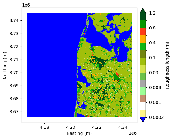
Next, let us visualize the roughness data, although remember the values on this chart will correspond to the landcover id, not to the roughness itself.
We have selected a colormap that has blue as its first color, since our first ID is water, however the other colors don’t necessarily correspond to the landcover classification that they correspond to. You could do more to specify the different colors by manipulating the colormap provided by Matplotlib.
[9]:
# Plot log of surface roughness lengths
cs = roughness.plot(figsize=(14, 10))

# Add the Høvsøre mast location
plt.plot(loc_x, loc_y, 'or', ms=16)

# Set the plot extent
plt.xlim([loc_x - plt_extent, loc_x + plt_extent])
plt.ylim([loc_y - plt_extent, loc_y + plt_extent]);
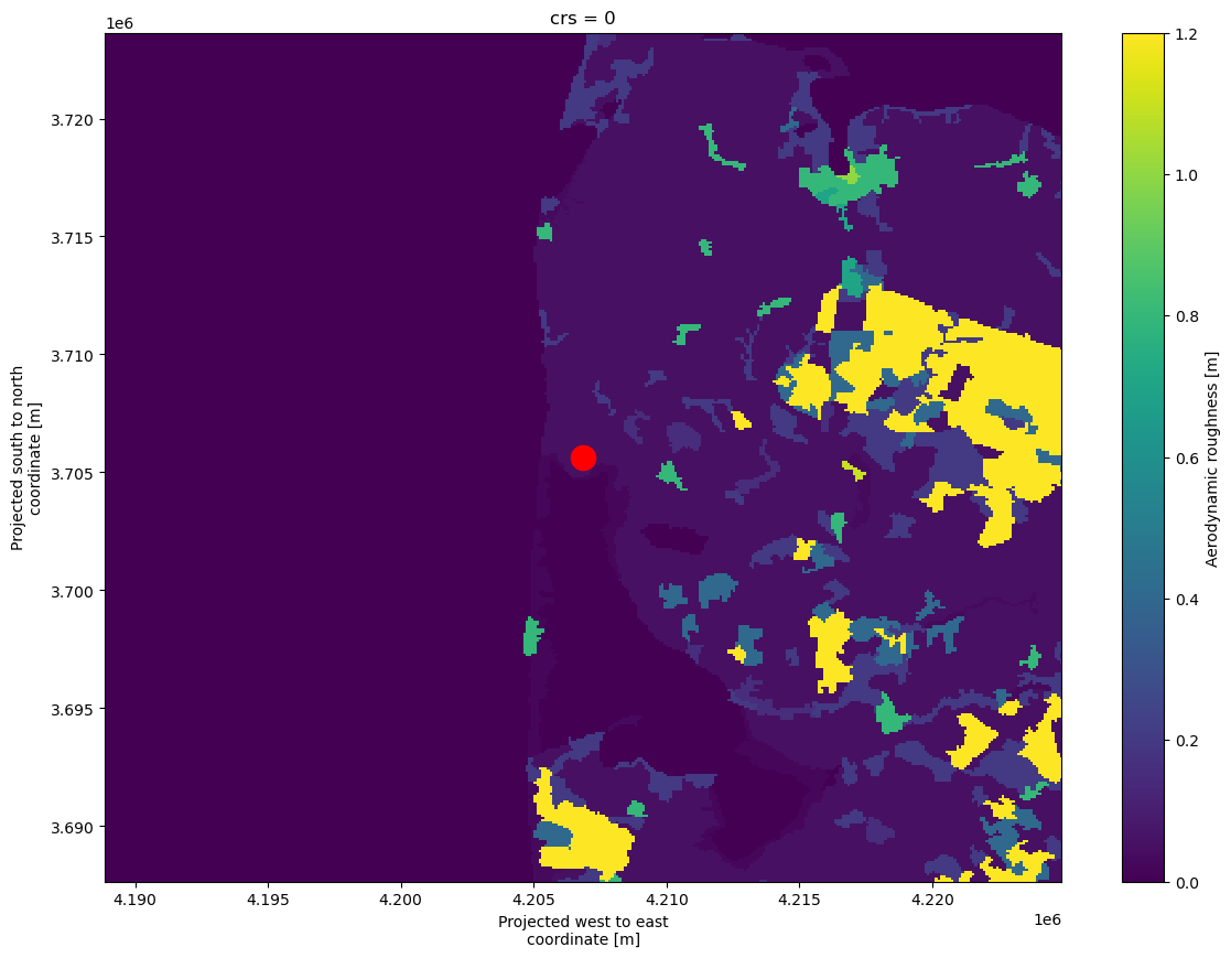
Again, we see the coastline clearly, and the water bodies south of the Høvsøre mast. To the east the plantation “Klosterhede plantage” is seen and north of it the city of “Lemvig”.
Site Effects#
The terrain data are used to calculate site effects used to generalize the observed wind climate (“going up” in WAsP lingo) and to downscale to nearby locations (“going down”).
The site effects are:
Orographic speed-up (by sector)
Internal boundar layer speed-up (by sector)
Effective upstream surface roughness (by sector)
pywasp note WAsP includes site effects due to obstacles, but we will not consider those here
Create TopographyMap object#
Let us investigate the site effects at the site. First we need to read in the raster data.
pywasp note
pywaspcan work with elevation raster maps directly
We will use elev.tif for the elevation. To convert the rasters, the pw.raster_to_vector function is used.
pywasp note: conversion to vector maps is a necessary step for roughness data, and recommended when you need to reproject elevation data.
[10]:
elev_map = pw.raster_to_vector(elev)
The vectormap is a geopandas.GeoDataFrame. Let’s inspect it.
[11]:
print(elev_map)
           elev                                           geometry
0      0.000000  LINESTRING (4205015.5 3686038.75, 4205015.5 36...
1      0.000000  LINESTRING (4226450.5 3718266, 4226450.5 37182...
2      0.000000  LINESTRING (4210436.5 3724936.25, 4210412 3724...
3      0.000000  LINESTRING (4209887 3724936.25, 4209812 372486...
4      0.000000  LINESTRING (4209737 3724936.25, 4209662.5 3724...
...         ...                                                ...
1214  62.299995  LINESTRING (4225348.5 3715792.75, 4225401 3715...
1215  71.199997  LINESTRING (4218955.5 3718246, 4218881 3718236...
1216  71.199997  LINESTRING (4221264 3718191, 4221279 3718183.5...
1217  71.199997  LINESTRING (4222448.5 3718041, 4222478 3718021...
1218  71.199997  LINESTRING (4223044 3718116, 4223078 3718103.7...

[1219 rows x 2 columns]
The GeoDataFrame contains two columns of data “elev” and “geometry”. The “elev” column holds the elevation height values and the “geometry” columns is a shapely.geometry.LINESTRING holding the spatial information of each elevation line.
We can use the builtin wk.plot.elevation_map method to visualize the elevation contours.
[12]:
wk.plot.elevation_map(elev_map, figsize=(3.5, 8))
[12]:
<Axes: title={'center': 'Elevation contour map'}, xlabel='Easting (m)', ylabel='Northing (m)'>

For the roughness data, a similiar conversion step is used.
[13]:
lc_map = pw.raster_to_vector(roughness)
[14]:
print(lc_map)
                                              geometry    z0
0    POLYGON ((4223300 3665700, 4223300 3665800, 42...  0.40
1    POLYGON ((4226100 3665700, 4226100 3665800, 42...  0.05
2    POLYGON ((4227200 3665700, 4227200 3665800, 42...  0.20
3    POLYGON ((4218600 3665700, 4218600 3665900, 42...  0.20
4    POLYGON ((4223200 3665700, 4223200 3666000, 42...  0.20
..                                                 ...   ...
989  POLYGON ((4239400 3745500, 4239400 3745600, 42...  0.20
990  POLYGON ((4238100 3730500, 4238100 3730800, 42...  0.05
991  POLYGON ((4221600 3731700, 4221600 3731800, 42...  0.05
992  POLYGON ((4223200 3745600, 4223200 3745700, 42...  0.80
993  POLYGON ((4227800 3744500, 4227800 3744600, 42...  0.20

[994 rows x 2 columns]
The vectormap contains a “geometry” that for a roughness or landcover map is made up of polygons. Each polygon has a corresponding roughness length z0.
Let us visualize the landcover-change contours using the wk.plot.polygon_map function.
[15]:
wk.plot.landcover_map(lc_map)
[15]:
<Axes: xlabel='Easting (m)', ylabel='Northing (m)'>
We can now use our elevation and landcover vectormaps to construct a pywasp TopographyMap object to calculate site effects.
[16]:
topo_map = pw.wasp.TopographyMap(elev_map, lc_map)
[17]:
topo_map
[17]:
Roughness map
                                              geometry    z0
0    POLYGON ((4223300 3665700, 4223300 3665800, 42...  0.40
1    POLYGON ((4226100 3665700, 4226100 3665800, 42...  0.05
2    POLYGON ((4227200 3665700, 4227200 3665800, 42...  0.20
3    POLYGON ((4218600 3665700, 4218600 3665900, 42...  0.20
4    POLYGON ((4223200 3665700, 4223200 3666000, 42...  0.20
..                                                 ...   ...
989  POLYGON ((4239400 3745500, 4239400 3745600, 42...  0.20
990  POLYGON ((4238100 3730500, 4238100 3730800, 42...  0.05
991  POLYGON ((4221600 3731700, 4221600 3731800, 42...  0.05
992  POLYGON ((4223200 3745600, 4223200 3745700, 42...  0.80
993  POLYGON ((4227800 3744500, 4227800 3744600, 42...  0.20

[994 rows x 2 columns]
Elevation map
           elev                                           geometry
0      0.000000  LINESTRING (4205015.5 3686038.75, 4205015.5 36...
1      0.000000  LINESTRING (4226450.5 3718266, 4226450.5 37182...
2      0.000000  LINESTRING (4210436.5 3724936.25, 4210412 3724...
3      0.000000  LINESTRING (4209887 3724936.25, 4209812 372486...
4      0.000000  LINESTRING (4209737 3724936.25, 4209662.5 3724...
...         ...                                                ...
1214  62.299995  LINESTRING (4225348.5 3715792.75, 4225401 3715...
1215  71.199997  LINESTRING (4218955.5 3718246, 4218881 3718236...
1216  71.199997  LINESTRING (4221264 3718191, 4221279 3718183.5...
1217  71.199997  LINESTRING (4222448.5 3718041, 4222478 3718021...
1218  71.199997  LINESTRING (4223044 3718116, 4223078 3718103.7...

[1219 rows x 2 columns]
Roughness Rose#
We will first explore the roughness elements upstream from the the Høvsøre mast for each of 12 sectors. We can do this by using get_rou_rose_pt method of topo_map, and pass in the location of the mast and the number of sectors we would like to use.
[18]:
rou_rose, _ = topo_map.get_rou_rose(bwc)
wk.plot.roughness_rose(rou_rose)
Data type cannot be displayed: application/vnd.plotly.v1+json
The open sea is clearly present to the west, and we see that the rose corresponds well to what we would expect from the roughness elements we saw in the map.
Output Locations#
Next up we will take a look at the site effects for the whole area surrounding the Høvsøre mast. We need to tell pywasp what locations we would like to calculate the site effects at. This is done by creating a xarray.Dataset with dimensions (west_east, south_north, and height) with coordinates values where we want to calculate the effects. Since this is a common need in PyWAsP, a convience function in pywasp.spatial called create_dataset has been created for this
purpose.
We tell pywasp that the projection of west_east, south_north coordinates are in the European grid projection by adding the coordinate reference system attribute crs="EPSG:3035".
numpy note we use
numpy’sarrayandlinspacearray constructors to pass in data arrays toxarray.Dataset.numpy.arraysimply takes a list of values and creates an array.numpy.linspacetakes a start and an end value, and the number of values to include linearly between them (including both ends).np.linspace(0, 5, 6)=np.array([0, 1, 2, 3, 4, 5])
[19]:
output_locs = wk.spatial.create_cuboid(
    np.linspace(loc_x-20000.0, loc_x+20000.0, 41).squeeze(),
    np.linspace(loc_y-20000.0, loc_y+20000.0, 41).squeeze(),
    np.array([100.0]),
    crs="EPSG:3035"
)
print(output_locs)
<xarray.Dataset> Size: 14kB
Dimensions:      (height: 1, south_north: 41, west_east: 41)
Coordinates:
  * height       (height) float64 8B 100.0
  * south_north  (south_north) float64 328B 3.686e+06 3.687e+06 ... 3.726e+06
  * west_east    (west_east) float64 328B 4.187e+06 4.188e+06 ... 4.227e+06
    crs          int8 1B 0
Data variables:
    output       (height, south_north, west_east) float64 13kB 0.0 0.0 ... 0.0
Attributes:
    Conventions:  CF-1.8
    history:      2025-07-04T13:12:01+00:00:\twindkit==1.0.0\t"cuboid")
Site Effects Calculation#
To get the site effects we will use the get_site_effects method from our topo_map object.
get_site_effects expects the unique west_east and south_north values, the number of sectors, and the height above ground, and the configuration object.
pywasp note depending on the number of locations,
get_site_effectsmay take some time to complete
[20]:
site_effects = topo_map.get_site_effects(output_locs, n_sectors=12)
print(site_effects)
<xarray.Dataset> Size: 1MB
Dimensions:              (sector: 12, south_north: 41, west_east: 41, height: 1)
Coordinates:
    crs                  int8 1B 0
    sector_ceil          (sector) float64 96B 15.0 45.0 75.0 ... 315.0 345.0
    sector_floor         (sector) float64 96B 345.0 15.0 45.0 ... 285.0 315.0
  * height               (height) float64 8B 100.0
  * south_north          (south_north) float64 328B 3.686e+06 ... 3.726e+06
  * west_east            (west_east) float64 328B 4.187e+06 ... 4.227e+06
  * sector               (sector) float64 96B 0.0 30.0 60.0 ... 300.0 330.0
Data variables: (12/15)
    z0meso               (sector, south_north, west_east) float32 81kB 0.0002...
    slfmeso              (sector, south_north, west_east) float32 81kB 0.0 .....
    displ                (sector, south_north, west_east) float32 81kB 0.0 .....
    flow_sep_height      (sector, south_north, west_east) float32 81kB 0.0 .....
    user_def_speedups    (sector, height, south_north, west_east) float32 81kB ...
    orographic_speedups  (sector, height, south_north, west_east) float32 81kB ...
    ...                   ...
    orographic_turnings  (sector, height, south_north, west_east) float32 81kB ...
    obstacle_turnings    (sector, height, south_north, west_east) float32 81kB ...
    roughness_turnings   (sector, height, south_north, west_east) float32 81kB ...
    site_elev            (south_north, west_east) float32 7kB 0.0 0.0 ... 0.0
    rix                  (south_north, west_east) float32 7kB 0.0 0.0 ... 0.0
    dirrix               (sector, south_north, west_east) float32 81kB 0.0 .....
Attributes:
    Conventions:      CF-1.8
    history:          2025-07-04T13:12:01+00:00:\twindkit==1.0.0\t"cuboid")\n...
    Package name:     windkit
    Package version:  1.0.0
    Creation date:    2025-07-04T13:12:04+00:00
    Object type:      Topographic effects
    author:           Bjarke Tobias Olsen
    author_email:     btol@dtu.dk
    institution:      DTU Wind
    title:            WAsP site effects
The site effects dataset is made up of following variables:
z0meso: effective upstream roughness by sectorslfmeso: effective upstream sea-land-fraction by sectordispl: displacement height by sectoruser_def_speedups: user defined speed-ups (as factor)orographic_speedups: speed-ups due to orography (as factor)obstacle_speedups: obstacle induced speed-ups (as factor)roughness_speedups: speed-ups due to roughness changes (as factor)user_def_turnings: user defined wind turning (in degrees)orographic_turnings: wind turning due to orography (in degrees)obstacle_turnings: wind turning due to obstracels (in degrees)roughness_turnings: wind turning due to roughness changes (in degrees)site_elev: surface elevationrix: ruggedness indexdirrix: sector wise ruggedness index
Plotting z0meso#
Let us take a look at the effective upstream surface roughness z0meso for the eastern sector (sector=90.0). We select this sector using xarray’s built-in selection method .sel. It is quite flexible and can take a single value .sel(sector=90.0) or a slice .sel(sector=slice(0.0, 180.0)). Here we just use 90.0.
We plot z0meso using xarray’s .plot method. We pass in figsize=(14, 10) to increase the size of the map.
We also plot the roughness map itself as a series of contour elements, to highlight the boundaries of the main roughness elements on the same map we also plot rgh. To get contour lines instead of filled contours, we explicitly ask for .plot.contour and tell it we want the colors to be white and the linestyles full (-).
We plot the location of the mast as before.
[21]:
site_effects['z0meso'].sel(sector=90.0).plot(figsize=(14, 10))
roughness.plot.contour(colors='white',add_labels=True, linestyles='-')
plt.plot(loc_x, loc_y, 'or', ms=16);
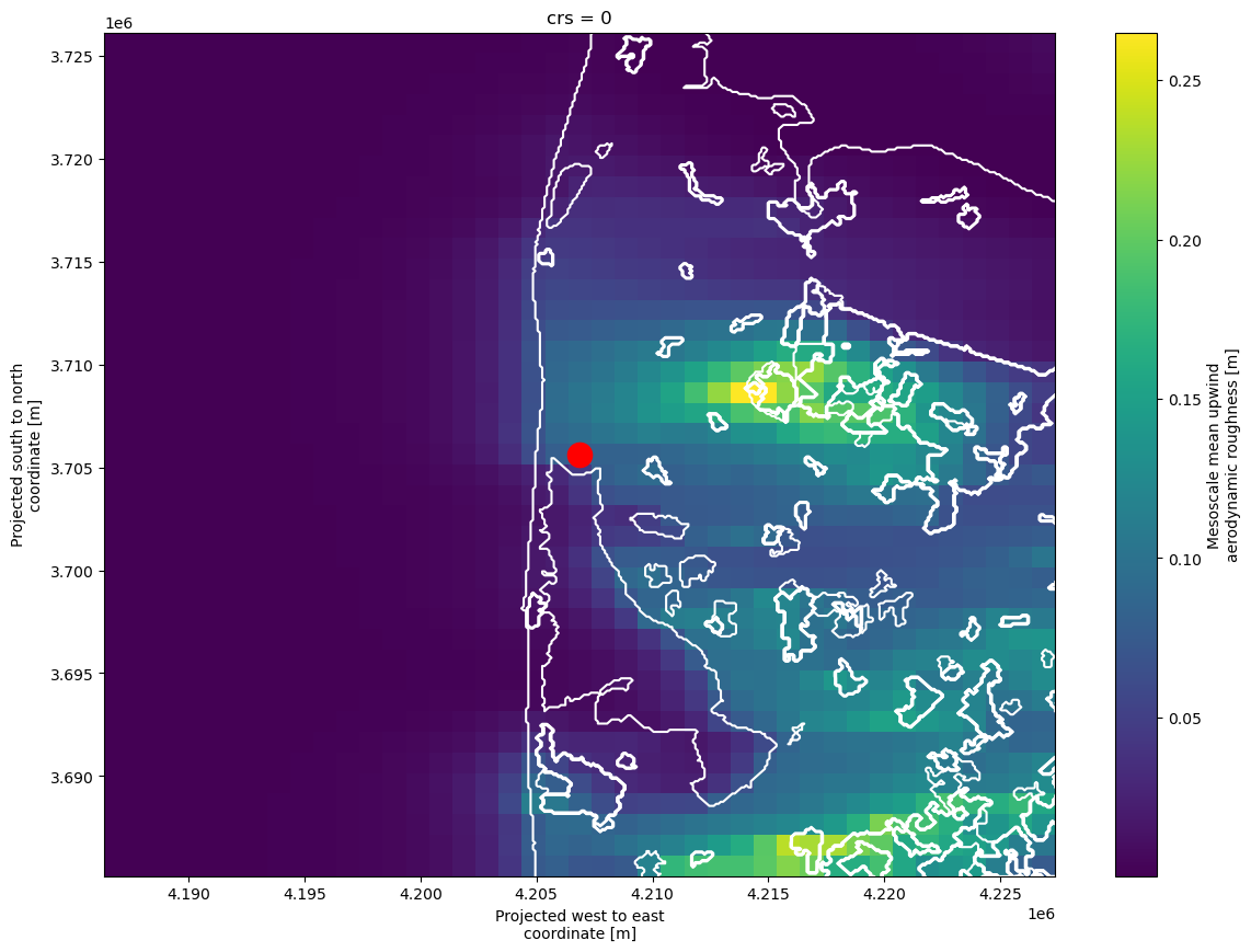
We clearly see the imprent of the plantation north-east of Høvsøre. We also see how the effective upstream roughness stays well above 0 for some distance offshore.
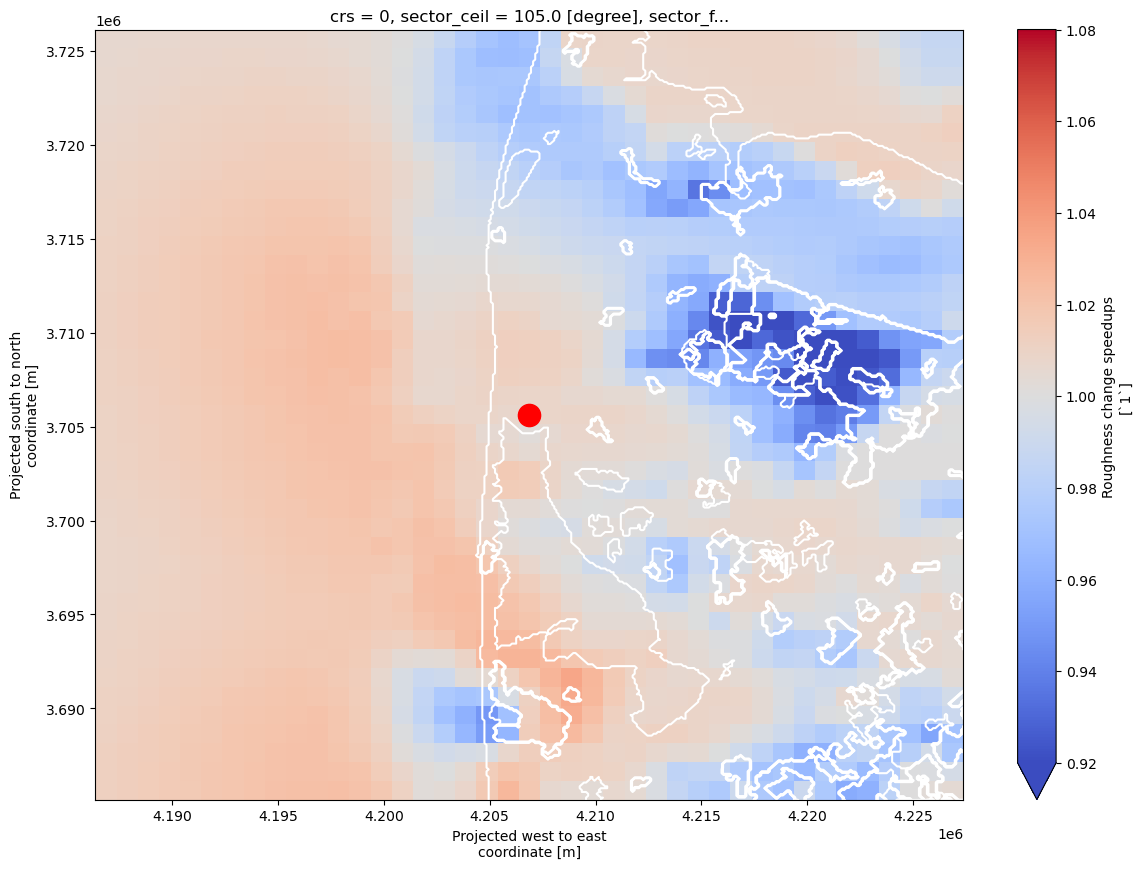
Plotting Roughness Change Speedups#
Next, let us investigate the speed-ups due to roughness changes.
Instead of using .sel to select by coordinate value, we will select by index using .isel. To get the same easterly direction we need to select sector index 3 - counting from 0. Python uses zero based indexing. xarray uses the name of the DataArray as the colorbar label, we can rename it to change that as well.
[22]:
(site_effects['roughness_speedups']
   .isel(sector=3)
   .rename(r'$DA_{rou}$ sector=90.0$^\circ$')
   .plot(vmin=0.92, vmax=1.08, cmap='coolwarm', figsize=(14, 10)))

roughness.plot.contour(colors='white', add_labels=False, linestyles='-')
plt.plot(loc_x, loc_y, 'or', ms=16);
Generalization and downscaling with PyWAsP#
Now it is time to actually generalize our observed wind climate and then downscale it to our chosen locations. Generalization involves calculating the wind speed for predefined surface roughnesses and heights above ground. So the first thing we need to do is chose these roughness and height classes.
Since we are prediction at 100 m, the default values of 10.0, 50.0, 100.0, 150.0, and 200.0 works fine.
[23]:
gen_heights = pw.wasp.derive_gen_heights()
print(gen_heights)
[10.0, 25.0, 50.0, 100.0, 250.0]
For roughness we can pass in the z0meso values to get an appropriate list of values.
[24]:
gen_roughnesses = pw.wasp.derive_gen_roughnesses(site_effects['z0meso'].values)
print(gen_roughnesses)
[0.0000000e+00 2.0523772e-04 1.8502603e-03 3.0101392e-02 3.9625481e-01]
The generalization is done with the generalize function from pywasp’s wasp module. It takes the binned wind climate (bwc), our topographic map (topo_map), the roughness and height classes, and finally the configuration object (conf).
[25]:
gwc = pw.wasp.generalize(bwc, topo_map, gen_roughnesses=gen_roughnesses, gen_heights=gen_heights)
print(gwc)
<xarray.Dataset> Size: 4kB
Dimensions:        (point: 1, sector: 12, gen_height: 5, gen_roughness: 5)
Coordinates:
    height         (point) float64 8B 100.0
    south_north    (point) float64 8B 3.706e+06
    west_east      (point) float64 8B 4.207e+06
    crs            int8 1B 0
    sector_ceil    (sector) float64 96B 15.0 45.0 75.0 ... 285.0 315.0 345.0
    sector_floor   (sector) float64 96B 345.0 15.0 45.0 ... 255.0 285.0 315.0
  * sector         (sector) float64 96B 0.0 30.0 60.0 90.0 ... 270.0 300.0 330.0
  * gen_roughness  (gen_roughness) float32 20B 0.0 0.0002052 ... 0.0301 0.3963
  * gen_height     (gen_height) float64 40B 10.0 25.0 50.0 100.0 250.0
Dimensions without coordinates: point
Data variables:
    A              (sector, gen_height, gen_roughness, point) float32 1kB 4.3...
    k              (sector, gen_height, gen_roughness, point) float32 1kB 1.3...
    wdfreq         (sector, gen_height, gen_roughness, point) float32 1kB 0.0...
    site_elev      (point) float32 4B 0.0
Attributes:
    Conventions:      CF-1.8
    history:          2025-07-04T13:11:55+00:00:\twindkit==1.0.0\tcreate_data...
    description:      Høvsøre observed wind climate EPSG:3035
    Package name:     windkit
    Package version:  1.0.0
    Creation date:    2025-07-04T13:12:06+00:00
    Object type:      Geostrophic Wind Climate
    author:           Bjarke Tobias Olsen
    author_email:     btol@dtu.dk
    institution:      DTU Wind
    title:            Generalized wind climate
The generalized wind climate contains weibull parameters (A and k) for each location, sector, and height and roughness class.
Predicted Wind Climates#
Now, let us calculate the wind climate at the location we have defined. The pywasp.wasp module provides two ways of doing this: downscale and downscale_from_site_effects. The latter assumes site effects that have already been calculated, while the first one will start by calculating them. Since we have already calculated the site effects, we will use downscale_from_site_effects. The function requires passing a interp_method. Two choices are available: given and
nearest. This is important when several generalized wind climates are present and will tell pywasp how to interpolate them to the location. Since just one wind climate is present in this study, the same generalized wind climate will be used everywhere.
After calculating the predicted wind climates at the output locations, we will enrich it by usefull derived quantities: the omnidirectional mean wind speed and power density. In Tutorial 4, we will show a way to calculate all of this in one pass.
[26]:
pwc = pw.wasp.downscale_from_site_effects(gwc, site_effects, interp_method='nearest')
[27]:
print(pwc)
<xarray.Dataset> Size: 250kB
Dimensions:       (sector: 12, height: 1, south_north: 41, west_east: 41)
Coordinates:
    crs           int8 1B 0
    sector_ceil   (sector) float64 96B 15.0 45.0 75.0 ... 285.0 315.0 345.0
    sector_floor  (sector) float64 96B 345.0 15.0 45.0 ... 255.0 285.0 315.0
  * height        (height) float64 8B 100.0
  * south_north   (south_north) float64 328B 3.686e+06 3.687e+06 ... 3.726e+06
  * west_east     (west_east) float64 328B 4.187e+06 4.188e+06 ... 4.227e+06
  * sector        (sector) float64 96B 0.0 30.0 60.0 90.0 ... 270.0 300.0 330.0
Data variables:
    A             (sector, height, south_north, west_east) float32 81kB 5.363...
    k             (sector, height, south_north, west_east) float32 81kB 1.346...
    wdfreq        (sector, height, south_north, west_east) float32 81kB 0.025...
    site_elev     (south_north, west_east) float32 7kB 0.0 0.0 0.0 ... 0.0 0.0
Attributes:
    Conventions:      CF-1.8
    history:          2025-07-04T13:12:01+00:00:\twindkit==1.0.0\t"cuboid")\n...
    Package name:     windkit
    Package version:  1.0.0
    Creation date:    2025-07-04T13:12:07+00:00
    Object type:      Geostrophic Wind Climate
    author:           Bjarke Tobias Olsen
    author_email:     btol@dtu.dk
    institution:      DTU Wind
    title:            WAsP site effects
The predicted wind climate contains the predicted probability density functions at the output locations. To enrich the wind climate with derived quantities, such as the mean wind speed or power density, pw.add_met_fields can be used.
[28]:
pwc = pw.add_met_fields(pwc)
print(pwc)
<xarray.Dataset> Size: 270kB
Dimensions:        (sector: 12, height: 1, south_north: 41, west_east: 41)
Coordinates:
    crs            int8 1B 0
    sector_ceil    (sector) float64 96B 15.0 45.0 75.0 ... 285.0 315.0 345.0
    sector_floor   (sector) float64 96B 345.0 15.0 45.0 ... 255.0 285.0 315.0
  * height         (height) float64 8B 100.0
  * south_north    (south_north) float64 328B 3.686e+06 3.687e+06 ... 3.726e+06
  * west_east      (west_east) float64 328B 4.187e+06 4.188e+06 ... 4.227e+06
  * sector         (sector) float64 96B 0.0 30.0 60.0 90.0 ... 270.0 300.0 330.0
Data variables:
    A              (sector, height, south_north, west_east) float32 81kB 5.36...
    k              (sector, height, south_north, west_east) float32 81kB 1.34...
    wdfreq         (sector, height, south_north, west_east) float32 81kB 0.02...
    site_elev      (south_north, west_east) float32 7kB 0.0 0.0 0.0 ... 0.0 0.0
    air_density    (height, south_north, west_east) float32 7kB 1.231 ... 1.234
    wspd           (height, south_north, west_east) float32 7kB 9.947 ... 9.497
    power_density  (height, south_north, west_east) float32 7kB 1.015e+03 ......
Attributes:
    Conventions:      CF-1.8
    history:          2025-07-04T13:12:01+00:00:\twindkit==1.0.0\t"cuboid")\n...
    Package name:     windkit
    Package version:  1.0.0
    Creation date:    2025-07-04T13:12:08+00:00
    Object type:      Met fields
    author:           Bjarke Tobias Olsen
    author_email:     btol@dtu.dk
    institution:      DTU Wind
    title:            WAsP site effects
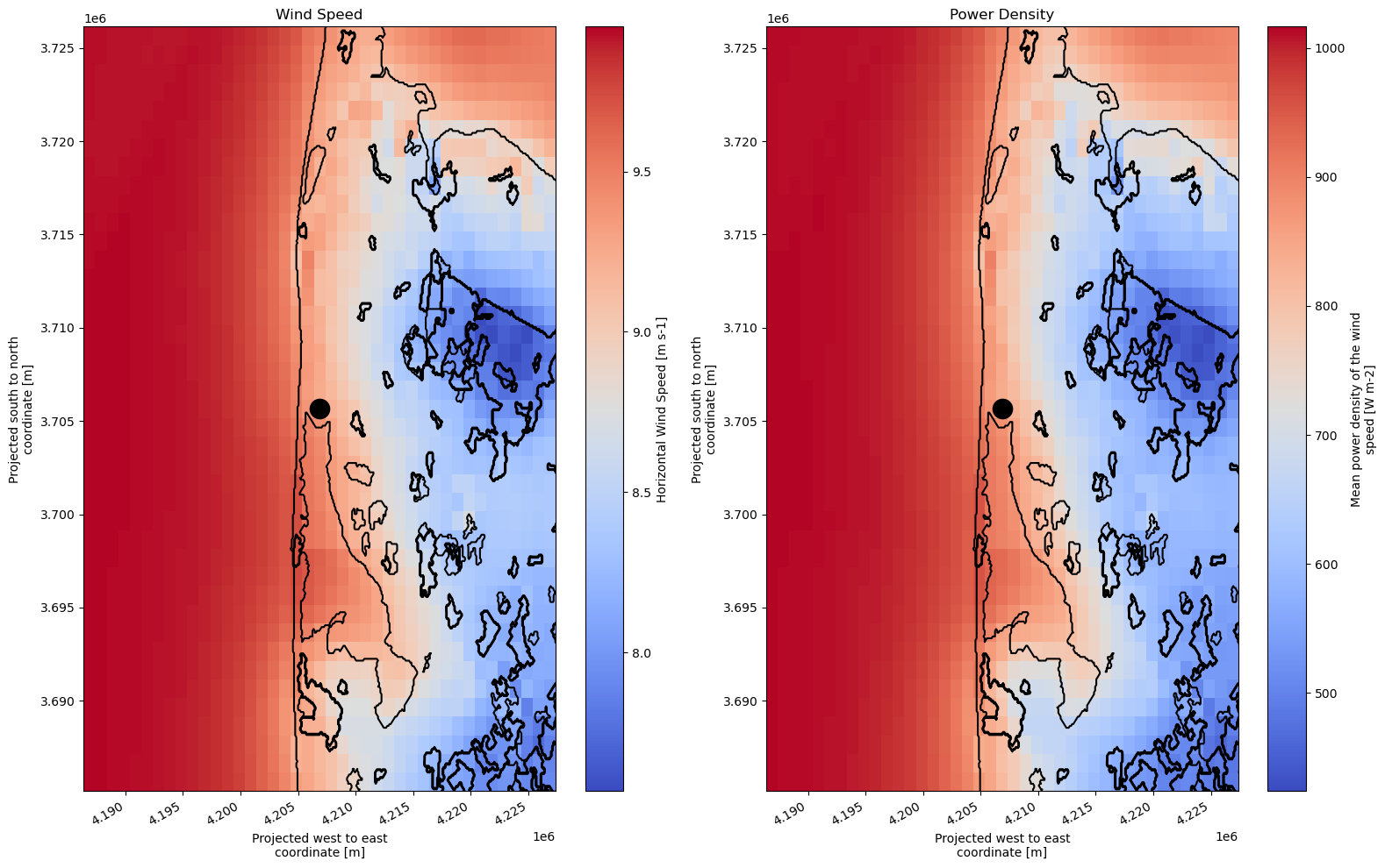
Finally the predicted wind climates around the site have been calculated. Let us plot the omnidirectional quantities: Weibull A and k, the mean wind speed, and the mean power density.
We will set up a plotting canvas consisting of four subplots using some matplotlib functionality. We define the subplots and pass their axes to the xarray plotting method when plotting the four quantities. Finally we add the roughness outlines and location of the mast.
[29]:
fig, axes = plt.subplots(1, 2, figsize=(16, 10))
ax1, ax2 = axes.flat

for var, ax in zip(pw.wasp.wind_climate.EMERGENT_FIELDS, axes.flat):
    pwc[var].isel(height=0).plot(ax=ax, cmap='coolwarm')

    roughness.plot.contour(colors='black', linestyles='-', ax=ax)
    ax.plot(loc_x, loc_y, 'ko', ms=16)
    plt.setp(ax.get_xticklabels(), rotation=30, horizontalalignment='right')

ax1.set_title("Wind Speed")
ax2.set_title("Power Density");

fig.tight_layout()