Understanding the BZ Orographic Model

Wind speeds change as air passes over hills, ridges, and valleys. The BZ model estimates these local orographic effects so that WAsP can remove them from an observed wind climate and apply them at a prediction site.

This tutorial focuses on the behavior that matters when preparing terrain and interpreting results. It uses a small synthetic hill to make the model response easy to see, followed by a compact example with real elevation data.

After working through the tutorial, you will be able to:

• explain why a hill can cause speed-up, slowdown, and flow turning;

• understand how the BZ model samples both nearby and distant terrain;

• interpret orographic speed-up, turning, and the ruggedness index (RIX);

• distinguish missing raster cells from sites outside a raster extent; and

• prepare a warped elevation raster before using it in a TopographyMap.

The BZ model in practical terms

The BZ model represents terrain as a combination of features with different horizontal scales. Each scale contributes to the wind response at the site: small nearby features mainly affect the flow close to the ground, while broader terrain features can influence the flow over greater distances and heights. Surface friction moderates that response near the ground.

For each requested site, the model samples terrain on a polar grid centered on that site. Samples are closely spaced nearby and progressively farther apart with distance. This zooming grid provides fine detail where it matters most while still including hills and valleys many kilometres away. It also means that terrain beyond the immediate raster cells around a site can affect the result.

The model returns two effects for each wind-direction sector:

• Orographic speed-up is a factor relative to the undisturbed wind. Values above 1 indicate speed-up and values below 1 indicate slowdown.

• Orographic turning is the terrain-induced change in wind direction.

The model is based on a linear description of near-neutral flow over terrain. It performs best over low and moderately sloped hills where the flow remains attached. Results require more caution on steep terrain, especially downstream of ridges where flow separation can occur. RIX helps identify such rugged terrain, but it is an indicator rather than a correction for every limitation.

from pathlib import Path
import matplotlib.pyplot as plt
import numpy as np
import pandas as pd
import windkit as wk
import xarray as xr
import pywasp as pw

CRS = 32632
N_SECTORS = 12
HEIGHT = 10.0
POINT_DIM = "stacked_point"

A Gaussian hill and four sites

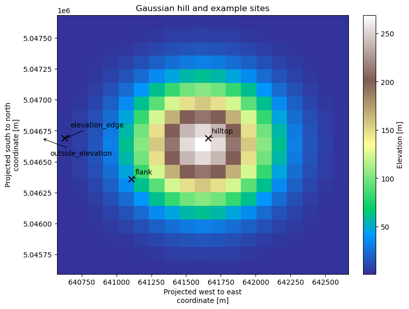
A smooth Gaussian hill makes the directional behavior easy to interpret. The four sites represent a hilltop, a lower flank, a point on the elevation-raster boundary, and a point just outside that boundary. The roughness map is uniform and extends beyond the elevation raster, so the example isolates orographic behavior. Sampling outside the elevation raster is not meaningful for a real modelling study; this point is included only to demonstrate the algorithm’s boundary handling.

hill_bounds = wk.spatial.create_dataset(
    west_east=[640629.5, 640629.5, 642629.5, 642629.5],
    south_north=[5045649.0, 5047649.0, 5045649.0, 5047649.0],
    height=HEIGHT,
    crs=CRS,
)
elevation = wk.create_raster_map(
    hill_bounds,
    resolution=110.0,
    map_type="elevation",
)

x = np.sort(elevation.west_east.values)
y = np.sort(elevation.south_north.values)
dx = float(x[1] - x[0])
dy = float(y[1] - y[0])
mid_x = len(x) // 2
mid_y = len(y) // 2

site_names = np.array(
    ["hilltop", "flank", "elevation_edge", "outside_elevation"],
    dtype=object,
)
sites = wk.spatial.create_dataset(
    west_east=[
        x[mid_x] + 0.35 * dx,
        x[len(x) // 4] + 0.35 * dx,
        x.min(),
        x.min() - 1.5 * dx,
    ],
    south_north=[
        y[mid_y] + 0.45 * dy,
        y[len(y) // 3] + 0.45 * dy,
        y[mid_y] + 0.45 * dy,
        y[mid_y] + 0.45 * dy,
    ],
    height=[HEIGHT],
    crs=CRS,
    struct="stacked_point",
).assign_coords({POINT_DIM: site_names})

plot_elevation_and_sites(elevation, sites, "Gaussian hill and example sites")

roughness_padding = 2.0 * max(dx, dy)
roughness_bbox = wk.spatial.BBox.from_bounds(
    float(x.min() - roughness_padding),
    float(y.min() - roughness_padding),
    float(x.max() + roughness_padding),
    float(y.max() + roughness_padding),
    crs=CRS,
)
roughness = wk.create_vector_map(
    roughness_bbox,
    map_type="roughness",
    roughness_change=(0.03, 0.03),
)
topography = pw.wasp.TopographyMap(elevation, roughness)

How the model sees the hill

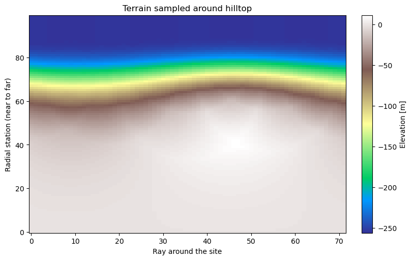
get_elev_rose exposes the terrain sampled around each site. In the plot below, each column is a ray pointing in a different direction and each row is a radial station. Radial station zero is close to the site; spacing increases outward. This representation is useful for understanding why the result is influenced by more than the nearest raster cells. The BZ grid is centred on the site, and each sampled terrain value is explicitly reported relative to the terrain elevation at that origin. These are therefore differences in site-relative terrain height, not differences in the map’s absolute datum. Note that because we are calculating at the top of a hill, the reported relative elevations in the BZ grid are negative.

elevation_rose = label_elevation_rose(
    topography.get_elev_rose(sites, n_sectors=N_SECTORS),
    sites,
)
plot_bz_grid(elevation_rose, "hilltop")

pd.DataFrame(
    {
        "site": site_names,
        "modelled site elevation [m]": elevation_rose["site_elev"].values,
        "RIX": elevation_rose["rix"].values,
    }
).set_index("site")

	modelled site elevation [m]	RIX
site
hilltop	257.000000	0.128336
flank	51.567497	0.037414
elevation_edge	3.000000	0.021933
outside_elevation	3.000000	0.017506

Directional speed-up and turning

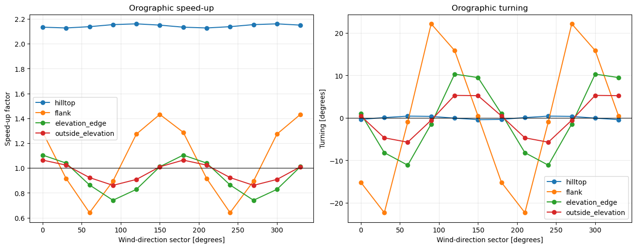
We now calculate the site effects at 10 m above ground. On a symmetric hill, the hilltop response is similar from opposite directions, while the flank is more directional. The boundary and outside points demonstrate that the model response depends on all terrain sampled around the site, not only on the cell directly underneath it.

get_site_effects uses one run from your PyWAsP subscription.

site_effects = topography.get_site_effects(sites, n_sectors=N_SECTORS)
plot_sectoral_effects(site_effects, site_names)

Preparing elevation rasters with missing cells

A raster cell containing NaN or infinity does not describe terrain. PyWAsP therefore refuses an elevation raster with such cells instead of guessing what lies there. The user must inspect the missing region and explicitly decide whether filling it is reasonable.

fill_elevation_nodata treats two common cases differently:

Missing-cell pattern	Fill method
Connected to the raster boundary	Nearest valid neighbour
Enclosed by valid cells	Piecewise-linear interpolation from surrounding cells

The function warns how many cells it fills. By default it also refuses to fill more than 5% of the raster, because a large no-data region may represent sea or missing coverage rather than a small reprojection artefact.

Boundary-connected missing cells

The following strip imitates missing cells introduced at an edge during raster processing. Constructing a TopographyMap from it produces an actionable error.

boundary_nan = elevation.astype(np.float32).copy(deep=True)
boundary_nan.values[mid_y - 3 : mid_y + 4, 0] = np.nan

try:
    pw.wasp.TopographyMap(boundary_nan, roughness)
except pw.PywaspError as error:
    print(error)

Elevation raster 'elevation' contains 7 NaN or Inf cell(s) (1.9% of the grid).  The WAsP core requires a clean grid.  Inspect the no-data regions; if they are small edge or reprojection artefacts, pre-fill them before building the TopographyMap:

    elev_map = windkit.fill_elevation_nodata(elev_map)

If instead they cover a large area (e.g. sea in a coastal DEM), trim the raster to its valid extent rather than filling it.

boundary_filled = wk.fill_elevation_nodata(boundary_nan)
plot_fill_result(
    boundary_nan,
    boundary_filled,
    "Boundary-connected cells filled from the nearest valid terrain",
)

/tmp/ipykernel_1332/805820126.py:1: UserWarning: Filling 7 boundary no-data cell(s) in elevation raster 'elevation' using nearest-neighbour interpolation.
  boundary_filled = wk.fill_elevation_nodata(boundary_nan)

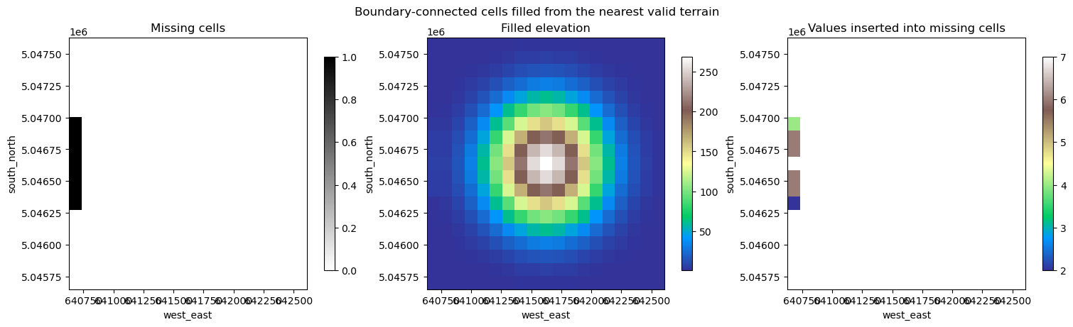
Filling changes cell values but not coordinates or raster extent. The outside_elevation site therefore remains outside the elevation raster; it is not turned into an inside site by the fill. These are separate behaviors: missing cells require an explicit decision. The outside site is evaluated only to demonstrate boundary handling; in a real study, every site should be covered by the elevation raster and its surrounding terrain.

filled_topography = pw.wasp.TopographyMap(boundary_filled, roughness)
filled_elevation_rose = label_elevation_rose(
    filled_topography.get_elev_rose(sites, n_sectors=N_SECTORS),
    sites,
)
plot_bz_grid_comparison(
    elevation_rose,
    filled_elevation_rose,
    "elevation_edge",
)

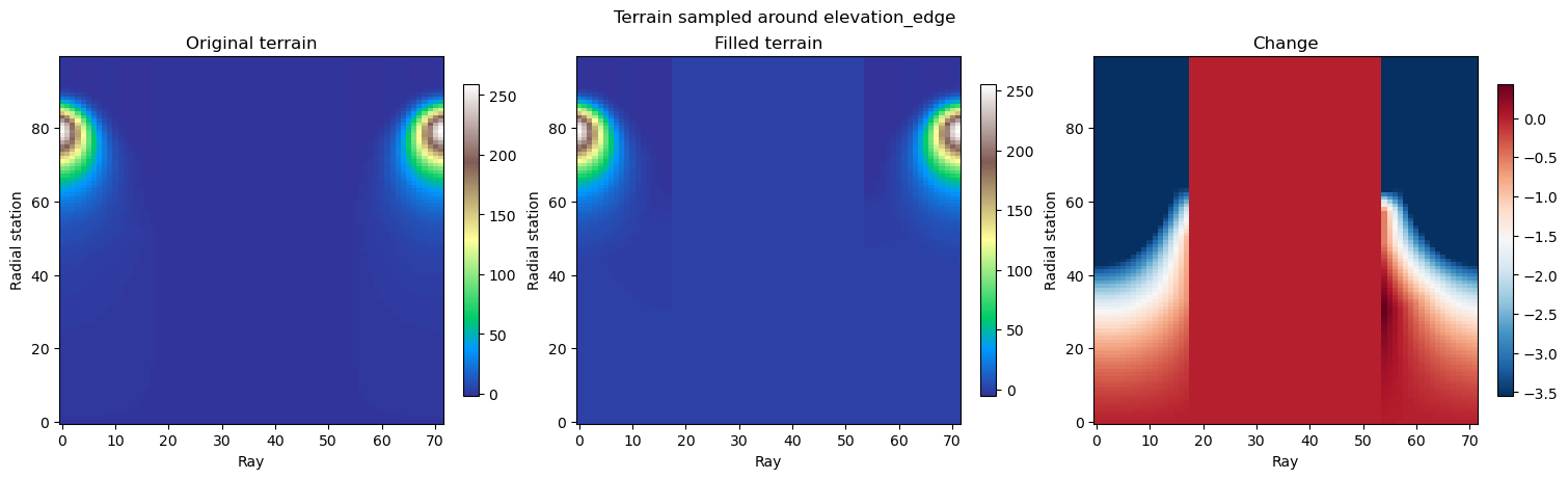
Reading the rightmost panel

The rightmost panel shows filled terrain - original terrain on the same BZ grid. If filling changes the origin’s site elevation, that reference-height change is included across the grid. A value of zero means the relative height at that ray and radial station is unchanged; positive and negative values show whether the filled terrain is higher or lower relative to the origin. The panel shows how the missing boundary strip changes terrain seen by the model, rather than showing a speed-up or turning result directly. Changes are seen in the easterly directions of the zooming grid, because the pixel were we report a value was filled with the nearest neighbour to the east (~7 m) instead of the true value (~3 m).

pd.DataFrame(
    {
        "site": site_names,
        "original RIX": elevation_rose["rix"].values,
        "RIX after fill": filled_elevation_rose["rix"].values,
        "site elevation after fill [m]": filled_elevation_rose["site_elev"].values,
    }
).set_index("site")

	original RIX	RIX after fill	site elevation after fill [m]
site
hilltop	0.128336	0.128336	257.000000
flank	0.037414	0.037414	51.567497
elevation_edge	0.021933	0.021933	6.550000
outside_elevation	0.017506	0.017506	6.550000

An enclosed missing cell

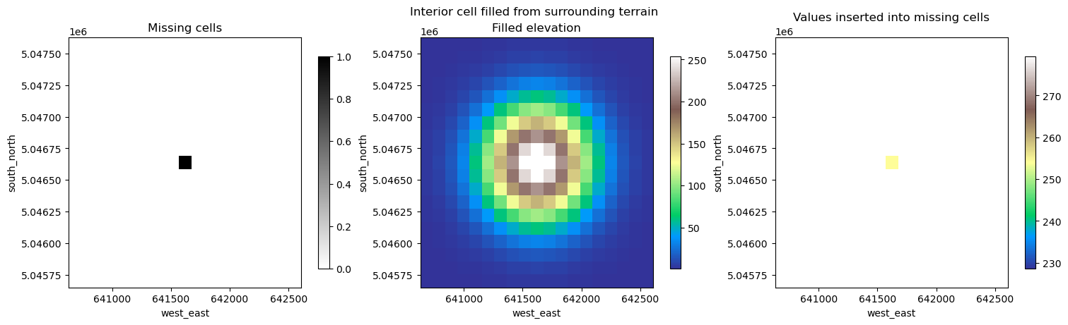
An isolated interior cell has valid terrain on every side, so interpolation is more appropriate than carrying the nearest value into the hole. Here we remove the summit cell, fill it explicitly, and confirm that the hill remains usable.

interior_nan = elevation.astype(np.float32).copy(deep=True)
interior_nan.values[mid_y, mid_x] = np.nan
interior_filled = wk.fill_elevation_nodata(interior_nan)

plot_fill_result(
    interior_nan,
    interior_filled,
    "Interior cell filled from surrounding terrain",
)

/tmp/ipykernel_1332/1407596901.py:3: UserWarning: Filling 1 interior no-data cell(s) in elevation raster 'elevation' using piecewise-linear interpolation.
  interior_filled = wk.fill_elevation_nodata(interior_nan)

interior_topography = pw.wasp.TopographyMap(interior_filled, roughness)
interior_elevation_rose = label_elevation_rose(
    interior_topography.get_elev_rose(sites, n_sectors=N_SECTORS),
    sites,
)
pd.DataFrame(
    {
        "site": site_names,
        "original RIX": elevation_rose["rix"].values,
        "RIX after interior fill": interior_elevation_rose["rix"].values,
    }
).set_index("site")

	original RIX	RIX after interior fill
site
hilltop	0.128336	0.128298
flank	0.037414	0.037414
elevation_edge	0.021933	0.021933
outside_elevation	0.017506	0.016908

A minimal real-terrain example

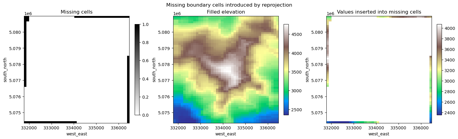
Reprojecting a geographic raster to a projected coordinate system usually produces a rectangular output whose corner cells lie outside the transformed source footprint. Those cells are commonly marked as missing. This example reads a compact 50×50 elevation raster centred on Mont Blanc, warps it to UTM zone 32N, and fills the resulting boundary artefacts. We read the bundled raster from disk for performance reasons; downloading the source raster makes this example slower and dependent on network access. Filling makes up terrain values from nearby valid cells, so it is only a compact way to demonstrate the workflow. For real modelling, the better solution is to extend the source map and use measured or otherwise valid terrain heights throughout the warped raster.

real_center = wk.spatial.create_point(
    west_east=6.8643,
    south_north=45.8326,
    height=100.0,
    crs=4326,
)
# To download the source raster instead, use these slower network-backed lines:
# elevation_bbox = wk.spatial.BBox.from_ds(real_center).buffer(0.007)
# geographic_elevation = wk.get_raster_map(elevation_bbox)

elevation_path = Path("data/mont_blanc_elevation.tif")
if not elevation_path.exists():
    elevation_path = Path(
        "modules/examples/tutorial_10/data/mont_blanc_elevation.tif"
    )
geographic_elevation = wk.read_elevation_map(elevation_path)
warped_elevation = wk.spatial.warp(geographic_elevation, CRS)

n_missing = int(np.isnan(warped_elevation.values).sum())
print(f"The warped raster contains {n_missing:,} missing boundary cells.")

real_elevation = wk.fill_elevation_nodata(warped_elevation)
plot_fill_result(
    warped_elevation,
    real_elevation,
    "Missing boundary cells introduced by reprojection",
)

The warped raster contains 122 missing boundary cells.

/tmp/ipykernel_1332/4293187801.py:22: UserWarning: Filling 122 boundary no-data cell(s) in elevation raster 'elevation' using nearest-neighbour interpolation.
  real_elevation = wk.fill_elevation_nodata(warped_elevation)

Practical guidance

• Use terrain data that extends far enough around every site to describe the hills and valleys that can influence it; you want at least a few kilometers of terrain elevation in all directions of a requested point.

• Inspect steep terrain and large RIX values as warning signs that the linearized model may be outside its strongest range of applicability.

• Treat missing cells as a data-quality decision. Fill small, understood gaps; trim or replace a raster with substantial missing coverage.

• Remember that filling missing values does not extend the raster coordinates. Check elevation and roughness coverage separately for all requested sites.

References

• Troen, I. (1990). A high resolution spectral model for flow in complex terrain. Proceedings of the European Community Wind Energy Conference.

• Troen, I. and Petersen, E. L. (1989). European Wind Atlas, Section 8.5, “The orographic model”. Risø National Laboratory.