

Grid Convergence and Wind-Direction Consistency#
Before reading this tutorial, read the WindKit grid-convergence example, which introduces true north, grid north, natural grid convergence, and effective grid convergence.
This tutorial focuses on the PyWAsP consequences: how direction reference frames affect binned wind climates, generalized wind climates, downscaling, direct prediction, and migration from older files.
Wind resource assessment depends on knowing which direction the wind is coming from. Direction is always measured relative to a north reference. In PyWAsP workflows that reference may be true north, the grid north of the map used for site effects, or the grid north of a mesoscale model. A 10-20 degree frame mismatch can shift energy between WAsP sectors and change roughness, shelter, or orographic corrections.
References
Hahmann, A. N. et al. (2020). The making of the New European Wind Atlas - Part 1: Model sensitivity. Geosci. Model Dev., 13, 5053-5078. https://gmd.copernicus.org/articles/13/5053/2020/
Global Wind Atlas: https://globalwindatlas.info/
Learning goals#
After working through this tutorial you will be able to:
Identify whether wind directions are true-north-relative or grid-relative before using them in PyWAsP.
Explain why WAsP sector bins make direction-frame errors visible in BWC, GWC, and WWC results.
Explain how the WRF
ALPHAvariable relates to the NEWA post-2018 direction-frame diagnosis.Describe how PyWAsP 2.1 stores
wind_dir_crs, uses automatic direction-frame alignment ingeneralize*,downscale*, andpredict_*workflows, and applies explicit alignment withalign_direction_crs(...).Choose a practical correction and migration strategy for old GWC/GeoWC files and WAsP GUI exports.
Part 1 - Why Grid Convergence Matters in PyWAsP#
The WindKit example covers the projection geometry. For PyWAsP, the operational issue is simpler: WAsP site effects are evaluated in sectors tied to the map or site-effect CRS, while input wind directions may arrive in a different frame.
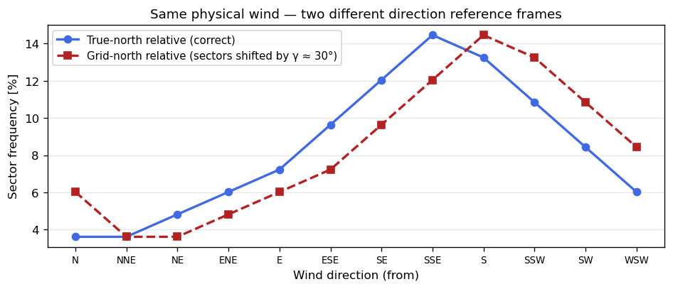
A binned wind climate (BWC) stores frequencies in discrete directional sectors, typically 12 sectors of 30 degrees. If a wind rose is true-north-relative but the site effects are grid-relative, the sector frequencies are applied to the wrong terrain directions. The correction must therefore be consistent with the CRS used for the map and site-effect calculation.
The figure below shows the practical effect: a frame rotation moves probability mass between sectors. That movement can change speedup and shelter corrections even when the wind speeds themselves are unchanged.
Part 2 - Historical Context: WRF, ALPHA, and NEWA#
2.1 WRF grid rotation and the ALPHA variable#
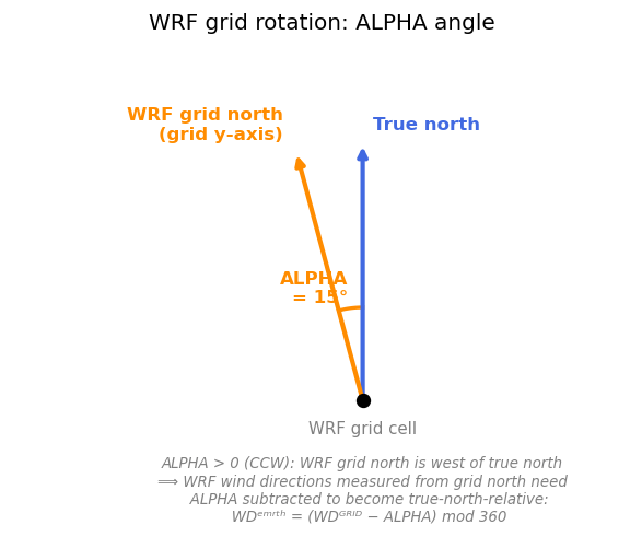
The WRF mesoscale model can store wind directions relative to its computational grid. For the New European Wind Atlas (NEWA), WRF was run with a Lambert Conformal Conic projection, and each grid cell includes ALPHA: the angle, in degrees and positive counter-clockwise, by which the WRF grid is rotated relative to geographic coordinates.
ALPHA uses the opposite sign from the WindKit/PyWAsP grid-convergence convention. A positive ALPHA means WRF grid north points west of true north. To convert WRF-grid-relative wind direction to true-north-relative direction, subtract ALPHA:
WD_earth = (WD_wrf - ALPHA) % 360
2.2 What is NEWA?#
The New European Wind Atlas (NEWA) is a mesoscale wind resource dataset for Europe produced with the WRF model at 3 km horizontal resolution. The original atlas covers 1989-2018 and is described in detail in Hahmann et al. (2020).
NEWA provides, at each grid cell and height level, half-hourly time series of wind speed and wind direction. The wind directions in the original dataset were correctly rotated from WRF grid-relative to true-north-relative using the per-cell ALPHA variable.
2.3 The manual 2019-2023 extension#
After 2018, the dataset was extended manually to 2024 to include the most recent data. During this update process an error was introduced: the wind direction rotation step was partially omitted. The wind directions for 2019-2023 were therefore stored grid-relative in WRF coordinates rather than true-north-relative. This error only becomes clear when you compare against an independent true-north-relative dataset such as ERA5 over the full period.
Part 3 - Diagnosing the error#
3.1 Time series of direction difference#
The analysis used a representative site in the far North-West (longitude ≈ −13 °, latitude ≈ 62 °, height 100 m) where the WRF ALPHA is large (~18 °). ERA5 wind directions at the same point serve as a reference.
The monthly-averaged difference between the NEWA (WRF) and ERA5 wind directions is plotted below — both for the corrected NEWA data and for the original uncorrected data.
When ERA5 is in true-north coordinates and NEWA is expressed in in grid-north coordinates, their direction difference should reflect the small residual between the two models’ dynamics. The mean of that difference should align with the mean local meridian convergence of the WRF projection at the site, which is shown with the red line.
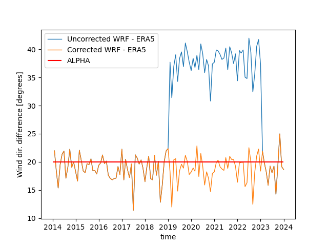
Figure 1. Monthly mean wind-direction difference (WRF − ERA5) at 100 m height for a site with large ALPHA (~18 °). The corrected line is stable over the full 1994–2024 period, meaning the physical relationship between the two datasets is consistent. The uncorrected line shows a step-change from 2019-2023 equal to roughly the local ALPHA value — the signature of the missing grid-to-earth rotation.
3.3 Using different projections#
As shown in the previous section it is easy to forget about the map rotation and just use the wind speed and direction without noticing anything strange. Usually in a WAsP context, you use the same map for the generalization and the downscaling. This was not the case for the New European Wind Atlas, where different maps were used for the generalization and downscaling, both with large meridian convergence angles.
However, for the microscale projection the proper meridian convergence was never treated correctly. This means that true-north relative generalized wind climates were used on a map with large meridian convergence. The impact of this is further illustrated in Part 6.
Part 4 - PyWAsP 2.1 Behavior#
PyWAsP 2.1 makes the direction reference frame explicit on BWC, GWC, and GeoWC datasets, and provides one alignment name in two places:
align_direction_crs=Trueis the automatic workflow option ondownscale*andpredict_*functions.pw.align_direction_crs(...)is the explicit helper for rotating an existing TSWC, BWC, WWC, or GWC into another direction CRS.bwc_from_tswc(..., wind_dir_crs=...)stores the projected grid frame used for binning.generalize*outputs always storewind_dir_crs.With
rotate_to_true_north=False, directions remain relative to the input grid andwind_dir_crsstores the projected source CRS WKT.With
rotate_to_true_north=True, directions are rotated to true north andwind_dir_crsstores the geodetic CRS WKT.predict_*functions use a BWCwind_dir_crsto align directions with the input map before applying the per-output downscale correction.
If a BWC has no wind_dir_crs, PyWAsP warns and assumes its directions are already relative to the input topography grid. A geographic BWC wind_dir_crs is rejected because generalization and prediction require grid-relative BWC directions. Older GWC/GeoWC files without metadata retain their backward-compatible downscaling behavior, but true-north files should be repaired before use. GeoWC is not supported by pw.align_direction_crs(...) because it contains additional geostrophic
variables that cannot be rotated by the WWC sector-rotation routine.
4.1 Affected APIs#
API family |
Direction-frame behavior |
|---|---|
|
With projected |
|
|
|
|
|
|
|
Explicitly rotates a TSWC, BWC, WWC, or GWC from |
The implementation uses WindKit’s grid_convergence(...) machinery internally. In PyWAsP terms, the important point is that wind_dir_crs records the source frame of stored BWC, GWC, and GeoWC directions, and automatic downscaling uses that frame to rotate directions into the output site-effect CRS. The explicit align_direction_crs(...) helper uses the same CRS-based rotation for standalone TSWC, BWC, WWC, and GWC datasets.
Part 5 - Recommended Workflows#
Option A: Direct prediction workflow
Use predict_bwc or predict_wwc when you do not need to inspect or store the intermediate GWC. Here we use adapt_gwc=False to match the equivalent generalize(..., rotate_to_true_north=False) plus downscale(..., align_direction_crs=True) workflow. With adapt_gwc=False, PyWAsP generalizes at the WAsP core’s classic heights [10, 25, 50, 100, 250], while generalize defaults to WAsP’s [10, 25, 50, 100, 200], so above 100 m the two only match if you pass
gen_heights=[10, 25, 50, 100, 250] to generalize. Generally you want to use adapt_gwc=False to avoid GWC lookup interpolation errors.
pwc = pw.wasp.predict_bwc(
    bwc,
    topo_map,
    target_locs,
    adapt_gwc=False,
    align_direction_crs=True,
)
Direct prediction first aligns a BWC with an explicit wind_dir_crs to the input map frame, then computes the downscale correction for each output location.
Option B: Two step workflow
For true-north-relative mast, lidar, or other observed time series, pass the projected topography CRS to bwc_from_tswc. It rotates directions into that map grid frame before binning and records wind_dir_crs on the BWC.
Then keep the default PyWAsP 2.1 behavior:
bwc = pw.bwc_from_tswc(tswc, wind_dir_crs=topo_map.elev_map.crs)

gwc = pw.wasp.generalize(
    bwc,
    topo_map,
    rotate_to_true_north=False,
)

wwc = pw.wasp.downscale(
    gwc,
    topo_map,
    target_locs,
    align_direction_crs=True,
)
When the same map projection is used for generalization and downscaling, the effective correction is approximately zero. The site effects and wind sectors stay in the same grid-relative frame.
Option C: Two-step true-north workflow
rotate_to_true_north=True is available when true-north GWC/GeoWC output is required for exchange or inspection. It can add extra sector interpolation compared with the primary grid-relative workflow, so it is usually not the preferred path for a local end-to-end PyWAsP calculation.
Imported true-north GWC/GeoWC workflow
Numerical wind atlases such as the Global Wind Atlas are commonly distributed with true-north-relative directions. Before downscaling such a GWC or GeoWC, make sure wind_dir_crs is a geodetic CRS WKT. Then leave align_direction_crs=True so the output directions are rotated into the target map grid frame.
Option D: Explicitly align a stored wind climate
Use pw.align_direction_crs(...) when you need a stored TSWC, BWC, WWC, or GWC in a specific direction frame before comparing, exporting, or reusing it. The helper requires an explicit source frame, either from wind_climate.attrs["wind_dir_crs"] or from source_wind_dir_crs=.
# True-north time series into the topography grid frame before binning.
tswc_grid = pw.align_direction_crs(
    tswc,
    target_wind_dir_crs=topo_map.elev_map.crs,
    source_wind_dir_crs=4326,
)
bwc = pw.bwc_from_tswc(tswc_grid, wind_dir_crs=topo_map.elev_map.crs)

# Existing climate with wind_dir_crs metadata into another grid frame.
bwc_target = pw.align_direction_crs(
    bwc,
    target_wind_dir_crs=wk.spatial.get_crs(target_locs),
)
Prefer aligning the least-compressed climate available. TSWC directions are rotated directly. BWC rotation is limited by sector and wind-speed-bin resolution. WWC and GWC are more compressed and can smear directional information because only sectoral Weibull parameters and frequencies remain. pw.align_direction_crs(...) does not support GeoWC.
Part 6 - Extreme Projection Demonstration#
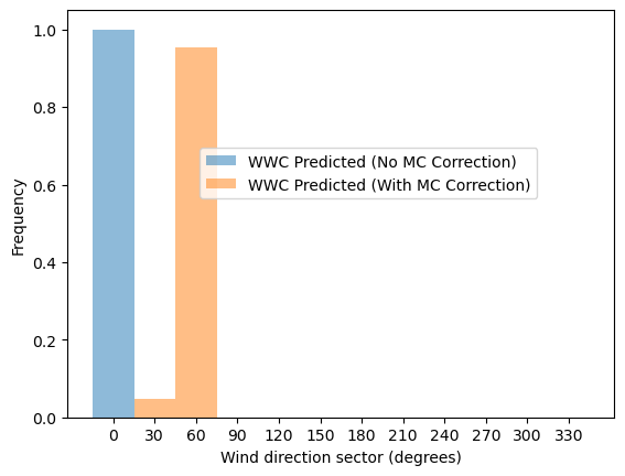
This executable example predicts and downscales a single-sector wind climate from UTM Zone 31N (EPSG:32631) to UTM Zone 41N (EPSG:32641) at 75 degrees N, 15 degrees E. These are intentionally extreme projections for the point; the purpose is to make the frame rotation easy to see.
The input BWC has 100% wind frequency in Sector 0. Without direction-frame correction, the peak stays in the original sector. With correction, the peak shifts by the inverse of the source-to-output grid-frame rotation. The direct site-effects prediction used here is equivalent to the direct predict_* path with adapt_gwc=False, and at this 100 m output height it should agree with generalize(..., rotate_to_true_north=False) + downscale(..., align_direction_crs=True).
[1]:
import sys

import matplotlib.pyplot as plt
import numpy as np
import windkit as wk

from pywasp import align_direction_crs
from pywasp.wasp.wind_atlas import (
    downscale_from_site_effects,
    generalize_from_site_effects,
    predict_wwc_from_site_effects,
)

# 1. Define coordinate reference systems (CRS) and location (75° N, 15° E)
pt_geo = wk.spatial.create_point(west_east=[15.0], south_north=[75.0], height=[100.0], crs=4326)
pt_32631 = wk.spatial.reproject(pt_geo, 32631)
pt_32641 = wk.spatial.reproject(pt_geo, 32641)

# 2. Calculate natural and effective grid-frame rotation
mc_in_natural = wk.spatial.grid_convergence(pt_32631).values[0]
mc_out_natural = wk.spatial.grid_convergence(pt_32641).values[0]
source_to_output_rotation = wk.spatial.grid_convergence(pt_32641, source=pt_32631).values[0]
# Downscaling applies the inverse grid-frame rotation to wind directions.
wind_direction_correction = -source_to_output_rotation

print(f"Input  (EPSG:32631) Natural MC: {mc_in_natural:+.4f}°")
print(f"Output (EPSG:32641) Natural MC: {mc_out_natural:+.4f}°")
print(f"Source-to-output grid-frame rotation: {source_to_output_rotation:+.4f}°")
print(f"Applied wind-direction correction: {wind_direction_correction:+.4f}° (clockwise plotted rotation)")
Input  (EPSG:32631) Natural MC: +11.6024°
Output (EPSG:32641) Natural MC: -47.0112°
Source-to-output grid-frame rotation: -58.6136°
Applied wind-direction correction: +58.6136° (clockwise plotted rotation)
[2]:
# 3. Create a single-sector BWC (100% wind frequency concentrated in Sector 0)
# We use a 12-sector BWC where Sector 0 is centered at 0° (range -15° to +15°)
bwc = wk.create_bwc(pt_32631, n_sectors=12, n_wsbins=20, not_empty=True).copy(deep=True)
bwc.attrs["wind_dir_crs"] = 32631  # Set the CRS for wind direction
bwc["wdfreq"][:] = 0.0
bwc["wdfreq"][0, 0] = 1.0

# Explicitly align the stored BWC into the output direction frame.
bwc_output_frame = align_direction_crs(bwc, target_wind_dir_crs=32641)

# 4. Create dummy Site Effects (flat terrain, open land z0 = 0.03)
def create_dummy_site_effects(ds):
    se = wk.create_wasp_site_effects(ds, n_sectors=12, not_empty=False, site_effects='all').copy(deep=True)
    se = se.fillna(0.0)
    se["user_def_speedups"][:] = 1.0
    se["orographic_speedups"][:] = 1.0
    se["obstacle_speedups"][:] = 1.0
    se["roughness_speedups"][:] = 1.0
    se["z0meso"][:] = 0.03
    return se

se_in = create_dummy_site_effects(pt_32631)
se_out = create_dummy_site_effects(pt_32641)
[3]:
# 5. Run direct WWC predictions (with and without direction-frame correction)
wwc_predict_no_mc = predict_wwc_from_site_effects(bwc, se_in, se_out, align_direction_crs=False)
wwc_predict_mc = predict_wwc_from_site_effects(bwc, se_in, se_out, align_direction_crs=True)

sectors = wwc_predict_no_mc.sector.values
bar_width = 30.0
plt.bar(sectors, wwc_predict_no_mc.wdfreq.values.flatten(), width=bar_width, alpha=0.5, label="WWC Predicted (No MC Correction)")
plt.bar(sectors, wwc_predict_mc.wdfreq.values.flatten(), width=bar_width, alpha=0.5, label="WWC Predicted (With MC Correction)")
plt.xticks(wwc_predict_no_mc.sector.values)
plt.xlabel("Wind direction sector (degrees)")
plt.ylabel("Frequency")
plt.legend(loc='center', bbox_to_anchor=(0.55, 0.6))
At line 555 of file ../../modules/waspcore/Rvea0288/Internal/generalization.f90
Fortran runtime warning: An array temporary was created for argument 'gd' of procedure 'gmom_ntb'
At line 555 of file ../../modules/waspcore/Rvea0288/Internal/generalization.f90
Fortran runtime warning: An array temporary was created for argument 'gf' of procedure 'gmom_ntb'
At line 586 of file ../../modules/waspcore/Rvea0288/Internal/generalization.f90
Fortran runtime warning: An array temporary was created for argument 'gd' of procedure 'gmom_ntb'
At line 586 of file ../../modules/waspcore/Rvea0288/Internal/generalization.f90
Fortran runtime warning: An array temporary was created for argument 'gf' of procedure 'gmom_ntb'
[3]:
<matplotlib.legend.Legend at 0x7ff03b73c6e0>
6.1 Geostrophic turning and residual probability mass#
The movement between the two WWC results is the meridian-convergence correction. The no-correction WWC can still retain probability in Sector 0; that residual is not a meridian-convergence effect. It comes from geostrophic turning and sector-model behaviour in WAsP, including interpolation on binned 30-degree sectors.
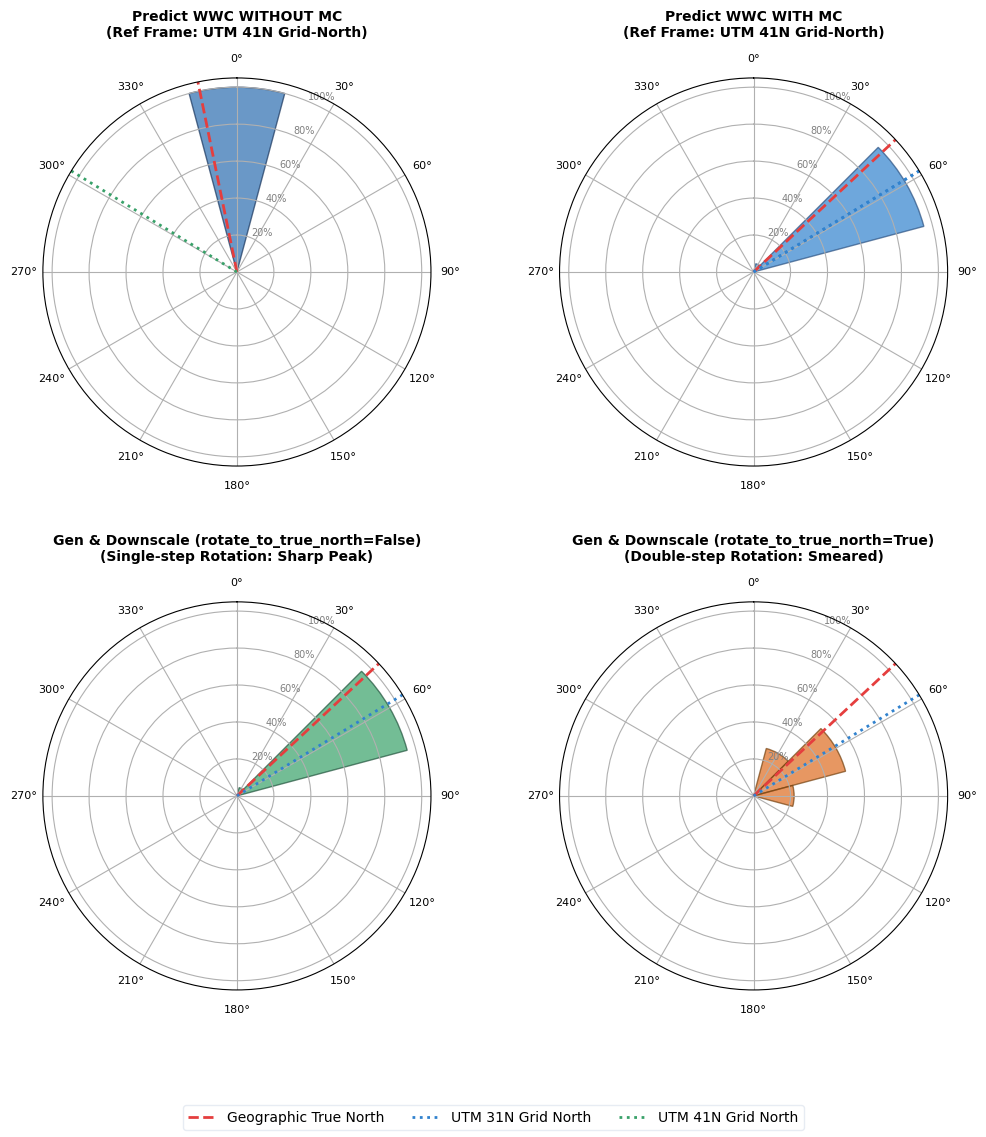
6.2 Single-step versus true-north two-step rotation#
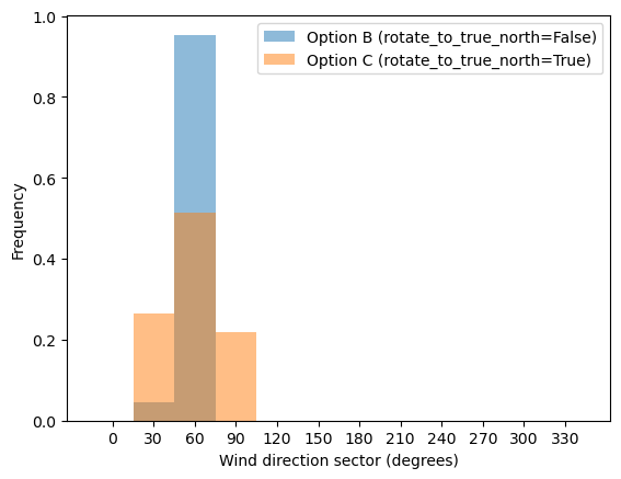
The comparison below keeps the PyWAsP-specific lesson visible. With rotate_to_true_north=False, the two-step workflow stores the source CRS in wind_dir_crs and applies one effective output correction during downscaling. With rotate_to_true_north=True, the workflow rotates to true north during generalization and then into the output grid during downscaling. Because these rotations act on binned sectors, the true-north two-step path can smear the wind rose more.
[4]:
# 6. Run Generalize & Downscale Workflows (Option B vs Option C)

# Option B: rotate_to_true_north=False (Recommended two-step workflow)
gwc_false = generalize_from_site_effects(bwc, se_in, rotate_to_true_north=False)
gwc_false_reprojected = wk.spatial.reproject(gwc_false, 32641)
wwc_false_mc = downscale_from_site_effects(gwc_false_reprojected, se_out, align_direction_crs=True)

# Option C: rotate_to_true_north=True (Two-step workflow via True North)
gwc_true = generalize_from_site_effects(bwc, se_in, rotate_to_true_north=True)
gwc_true_reprojected = wk.spatial.reproject(gwc_true, 32641)
wwc_true_mc = downscale_from_site_effects(gwc_true_reprojected, se_out, align_direction_crs=True)

max_abs_diff = float(np.nanmax(np.abs(wwc_predict_mc.wdfreq.values - wwc_false_mc.wdfreq.values)))
print(f"Max abs frequency difference, direct WWC vs grid-relative two-step: {max_abs_diff:.3e}")

sectors = wwc_false_mc.sector.values
bar_width = 30.0
plt.bar(sectors, wwc_false_mc.wdfreq.values.flatten(), width=bar_width, alpha=0.5, label="Option B (rotate_to_true_north=False)")
plt.bar(sectors, wwc_true_mc.wdfreq.values.flatten(), width=bar_width, alpha=0.5, label="Option C (rotate_to_true_north=True)")
plt.xticks(wwc_false_mc.sector.values)
plt.xlabel("Wind direction sector (degrees)")
plt.ylabel("Frequency")
plt.legend();
Max abs frequency difference, direct WWC vs grid-relative two-step: 0.000e+00
6.3 Polar comparison#
The polar plots below are drawn in local grid-relative frames because that is the frame used by WAsP site effects. The dashed reference lines show how the same physical direction appears under the two projection grids.
[5]:
# 12 sectors, centered at 0, 30, 60, ..., 330 degrees
angles_rad = np.radians(np.arange(0, 360, 30))

# Extract the frequency values from xarray objects for the custom polar visualization
freq_wwc_no_mc = wwc_predict_no_mc.wdfreq.values.flatten()
freq_wwc_mc = wwc_predict_mc.wdfreq.values.flatten()
freq_false_mc = wwc_false_mc.wdfreq.values.flatten()
freq_true_mc = wwc_true_mc.wdfreq.values.flatten()

fig, axs = plt.subplots(2, 2, figsize=(12, 12), subplot_kw={'projection': 'polar'})

# Helper to configure polar plot aesthetics
def setup_polar_ax(ax, title):
    ax.set_theta_zero_location("N")
    ax.set_theta_direction(-1) # Clockwise
    ax.set_title(title, fontsize=10, pad=12, weight='bold')
    ax.set_xticks(np.radians(np.arange(0, 360, 30)))
    ax.set_xticklabels([f"{d}°" for d in range(0, 360, 30)], fontsize=8)
    ax.set_ylim(0, 1.05)
    ax.set_yticks([0.2, 0.4, 0.6, 0.8, 1.0])
    ax.set_yticklabels(["20%", "40%", "60%", "80%", "100%"], fontsize=7, color="gray")

# Panel 1: Predict WWC WITHOUT MC
setup_polar_ax(axs[0, 0], "Predict WWC WITHOUT MC\n(Ref Frame: UTM 41N Grid-North)")
axs[0, 0].bar(angles_rad, freq_wwc_no_mc, width=np.radians(30), bottom=0.0,
              edgecolor='#1a365d', facecolor='#2b6cb0', alpha=0.7)
line_tn = axs[0, 0].axvline(np.radians(-mc_in_natural), color='#e53e3e', linestyle='--', linewidth=2, label="Geographic True North")
line_out_n = axs[0, 0].axvline(np.radians(source_to_output_rotation), color='#38a169', linestyle=':', linewidth=2, label="UTM 41N Grid North")

def add_reference_lines_output(ax):
    ax.axvline(np.radians(-mc_out_natural), color='#e53e3e', linestyle='--', linewidth=2)
    ax.axvline(np.radians(wind_direction_correction), color='#3182ce', linestyle=':', linewidth=2)

# Panel 2: Predict WWC WITH MC
setup_polar_ax(axs[0, 1], "Predict WWC WITH MC\n(Ref Frame: UTM 41N Grid-North)")
axs[0, 1].bar(angles_rad, freq_wwc_mc, width=np.radians(30), bottom=0.0,
              edgecolor='#2c5282', facecolor='#3182ce', alpha=0.7)
add_reference_lines_output(axs[0, 1])
line_in_n = axs[0, 1].axvline(np.radians(wind_direction_correction), color='#3182ce', linestyle=':', linewidth=2, label="UTM 31N Grid North")

# Panel 4: Part C (Gen & Downscale, Option B)
setup_polar_ax(axs[1, 0], "Gen & Downscale (rotate_to_true_north=False)\n(Single-step Rotation: Sharp Peak)")
axs[1, 0].bar(angles_rad, freq_false_mc, width=np.radians(30), bottom=0.0,
              edgecolor='#22543d', facecolor='#38a169', alpha=0.7)
add_reference_lines_output(axs[1, 0])

# Panel 5: Part D (Gen & Downscale, Option C)
setup_polar_ax(axs[1, 1], "Gen & Downscale (rotate_to_true_north=True)\n(Double-step Rotation: Smeared)")
axs[1, 1].bar(angles_rad, freq_true_mc, width=np.radians(30), bottom=0.0,
              edgecolor='#744210', facecolor='#dd6b20', alpha=0.7)
add_reference_lines_output(axs[1, 1])

fig.legend(handles=[line_tn, line_in_n, line_out_n], loc='lower center',
           ncol=3, fontsize=10, frameon=True, facecolor='white', edgecolor='#e2e8f0')

plt.subplots_adjust(bottom=0.12, hspace=0.35, wspace=0.25)
Part 7 - Practical Checklist#
Check whether every input direction dataset is true-north-relative or grid-relative before ingestion.
For true-north observed time series, call
bwc_from_tswc(..., wind_dir_crs=topo_map.elev_map.crs)so the BWC is explicitly grid-relative before generalization or prediction.Leave
align_direction_crs=Trueunless you are intentionally reproducing legacy behavior.For the primary two-step workflow, use the default
generalize(..., rotate_to_true_north=False)followed bydownscale(..., align_direction_crs=True).When you want the
predict_bwcresult to match the equivalent two-step workflow, usepredict_bwcorpredict_wwcwithadapt_gwc=Falseand the default direction-frame alignment. Above 100 m, also passgen_heights=[10, 25, 50, 100, 250]togeneralize.Verify or repair
wind_dir_crson old GWC/GeoWC files before downscaling. For TSWC, BWC, WWC, or GWC, usepw.align_direction_crs(...)when you need to convert a stored climate to a target direction frame explicitly.Compare predicted climates and observations in the same direction frame. Align one of them first if needed.
Part 8 - Migration Guide: PyWAsP < 2.1 and WAsP GUI Wind Climates#
GWC and GeoWC files produced before PyWAsP 2.1, or exported from WAsP GUI, may not contain wind_dir_crs. Without this attribute PyWAsP cannot know whether stored directions are true-north-relative or grid-relative. For backward compatibility, align_direction_crs=True falls back to no rotation when the attribute is absent.
That fallback is appropriate for many old WAsP GUI workflows where the GWC was created and reused in the same projected map frame. It is not appropriate for imported true-north GWC/GeoWC files, such as files from numerical wind atlas workflows, when downscaling on a projected microscale map.
Set or repair wind_dir_crs before downscaling:
import pyproj
import pywasp as pw
import windkit as wk

gwc = wk.read_gwc("my_old_atlas.gwc")

# True-north-relative GWC/GeoWC: store a geodetic CRS WKT.
gwc.attrs["wind_dir_crs"] = pyproj.CRS.from_epsg(4326).to_wkt()

wwc = pw.wasp.downscale(
    gwc,
    topo_map,
    target_locs,
    align_direction_crs=True,
)
For a grid-relative old file, store the projected CRS WKT of the map or site effects that define the wind-direction frame:
gwc.attrs["wind_dir_crs"] = wk.spatial.get_crs(site_effects).to_wkt()
If you are deliberately reproducing legacy behavior, set align_direction_crs=False or leave wind_dir_crs absent. Otherwise, make the direction CRS explicit. For old BWC, WWC, or GWC files with a known source frame, pw.align_direction_crs(...) can also rewrite the climate into the target frame before later use. GeoWC files should be repaired by setting wind_dir_crs metadata and then downscaled with align_direction_crs=True.
Glossary#
Term |
Definition |
|---|---|
``wind_dir_crs`` |
Attribute on BWC, GWC, and GeoWC datasets that records the CRS frame of stored wind directions. BWC values must be projected CRS WKT strings; GWC/GeoWC may also use geodetic CRS WKT strings for true-north-relative directions. |
``rotate_to_true_north`` |
|
``align_direction_crs=True`` |
|
``pw.align_direction_crs(…)`` |
Explicit helper that rotates TSWC, BWC, WWC, or GWC directions from |
Grid-relative BWC/GWC/WWC |
A wind climate whose directions are measured from the grid north of a specific projected CRS. |
True-north-relative GWC/GeoWC |
A generalized or geostrophic wind climate whose directions are measured from geographic true north and whose |
WRF ``ALPHA`` |
Per-cell WRF grid-rotation angle, positive counter-clockwise. For NEWA diagnosis, missing ALPHA correction leaves WRF-grid-relative directions in files expected to be true-north-relative. |
Appendix A - Internal Direction-Rotation Notes#
From PyWAsP 2.1, bwc_from_tswc(..., wind_dir_crs=...) creates an explicitly grid-relative BWC, and every GWC produced by generalize_from_site_effects() and every GeoWC produced by generalize_from_site_effects_to_geowc() carries wind_dir_crs.
Attribute value |
Meaning |
|---|---|
Geodetic CRS WKT |
Directions are true-north-relative. |
Projected CRS WKT |
Directions are relative to that projection’s grid north. |
absent |
Older file; reference frame unknown. |
The default rotate_to_true_north=False records the input site-effect CRS in wind_dir_crs. A later downscale can then compute the output correction even if the GWC has been reprojected, because wind_dir_crs records the original direction frame rather than the dataset’s current coordinate CRS.
The public rotation helpers used internally, such as pw.wwc_rotate and pw.bwc_resample_sectors, can also be useful when validating results against observations in a different direction frame.
Appendix B - Direction-sign conventions in the Part 6 example#
This appendix uses the same 100% north wind climate from Part 6. The input BWC has all probability in sector 0, and bwc.attrs["wind_dir_crs"] says that sector 0 is measured relative to UTM 31N grid north.
The important distinction is:
grid_convergence(...)returns a north-frame rotation.Wind-direction sector numbers transform with the opposite sign, because the reference axis moves while the physical direction does not.
B.1 Natural versus effective grid convergence#
For a single CRS, grid_convergence(ds) is the rotation from true north to that CRS grid north:
gamma_crs = grid_north_crs - true_north
With source=, WindKit returns the frame rotation from the source CRS grid north to the target CRS grid north, evaluated at the target locations:
source_to_target = gamma_target - gamma_source
That is the value used by align_direction_crs=True when moving a GWC from its stored direction frame into the output site-effect frame. The explicit pw.align_direction_crs(...) helper uses the same sign convention when rewriting a stored TSWC, BWC, WWC, or GWC into a target direction frame.
[6]:
print(f"Input  UTM 31N natural convergence:  {mc_in_natural:+.4f}°")
print(f"Output UTM 41N natural convergence:  {mc_out_natural:+.4f}°")
print(f"Output minus input:                  {mc_out_natural - mc_in_natural:+.4f}°")
print(f"grid_convergence(output, source=input): {source_to_output_rotation:+.4f}°")
print()
print("Wind direction numbers use the opposite sign:")
print(f"  source-to-output frame rotation:   {source_to_output_rotation:+.4f}°")
print(f"  applied direction correction:      {wind_direction_correction:+.4f}°")
Input  UTM 31N natural convergence:  +11.6024°
Output UTM 41N natural convergence:  -47.0112°
Output minus input:                  -58.6136°
grid_convergence(output, source=input): -58.6136°

Wind direction numbers use the opposite sign:
  source-to-output frame rotation:   -58.6136°
  applied direction correction:      +58.6136°
B.2 Why the corrected peak moves from north#
The Part 6 BWC is deliberately simple: 100% frequency in sector 0. That means “wind from north” in the input direction frame, i.e. UTM 31N grid north.
When downscaling to UTM 41N with align_direction_crs=True, PyWAsP computes the effective input-grid to output-grid frame rotation and applies the inverse direction correction:
wd_output = (wd_input - source_to_output_rotation) % 360
For this example wd_input = 0°, so the expected output direction is exactly wind_direction_correction % 360. Because the climate is binned in 30° sectors, the plotted peak appears in the nearest sector center rather than at the exact continuous angle.
[7]:
input_peak_direction = 0.0
expected_output_direction = (input_peak_direction - source_to_output_rotation) % 360.0

def peak_sector_from_wdfreq(wc):
    wdfreq = wc.wdfreq.squeeze(drop=True)
    return float(wdfreq.sector.isel(sector=np.argmax(wdfreq.values)))

print(f"Input BWC peak direction:                    {input_peak_direction:7.3f}°")
print(f"Expected continuous output direction:        {expected_output_direction:7.3f}°")
print(f"Explicitly aligned BWC sector center:        {peak_sector_from_wdfreq(bwc_output_frame):7.3f}°")
print(f"Nearest corrected predict_wwc sector center: {peak_sector_from_wdfreq(wwc_predict_mc):7.3f}°")
print(f"No-correction predict_wwc sector center:     {peak_sector_from_wdfreq(wwc_predict_no_mc):7.3f}°")
Input BWC peak direction:                      0.000°
Expected continuous output direction:         58.614°
Explicitly aligned BWC sector center:         60.000°
Nearest corrected predict_wwc sector center:  60.000°
No-correction predict_wwc sector center:       0.000°
B.3 Function sign summary#
Function or workflow |
Sign convention |
|---|---|
|
True-north to |
|
Source-grid to target-grid frame rotation: |
Direction-number conversion |
Opposite sign from the frame rotation: |
|
Keeps the GWC in the input map/grid frame and stores that frame in |
|
Computes |
|
Same net convention as the grid-relative two-step workflow: align input to the input map frame, then apply the inverse source-to-output correction. |
|
Rewrites TSWC, BWC, WWC, or GWC directions into the target frame with the same inverse direction-number convention and updates |
In Part 6, this is why the corrected 100% north climate moves by -source_to_output_rotation, while the uncorrected case stays near sector 0.