Long-Term Correction with MCP

This example shows how to perform a Measure-Correlate-Predict (MCP) long-term correction using LinRegMCP and VarRatMCP.

The workflow is:

1. A long-term (LT) reference station provides many years of wind data.

2. Short-term (ST) target on-site measurements that overlap the reference data (concurrent period).

3. An MCP model is fitted on the concurrent period, mapping reference wind speeds to site wind speeds sector by sector.

4. The fitted model is applied to the full long-term reference to produce a long-term corrected site wind climate.

Generate Synthetic Data

import numpy as np
import matplotlib.pyplot as plt
import pandas as pd
import windkit as wk
from windkit.ltc import LinRegMCP, VarRatMCP, calc_scores
from windkit.spatial import create_point

out_locs = create_point(500000, 6200000, 80, 32632)

period_lt = pd.date_range("2004-01-01", "2009-01-01", freq="1h", inclusive="left")
period_st = pd.date_range("2008-01-01", "2009-01-01", freq="1h", inclusive="left")

# Generation of synthetic data for a correlated pair, with same direction bias.
tgt_lt, ref_lt = wk.create_tswc_pair(
    out_locs,
    date_range=period_lt,
    weibull_A=(6.0, 8.0),
    weibull_k=(1.6, 2.2),
    target_r2=0.8,
    direction_bias=0,
    speed_tau=14400.0,  # set the e-folding timescale for the wind speed
)
ref_st, tgt_st = ref_lt.sel(time=period_st), tgt_lt.sel(time=period_st)

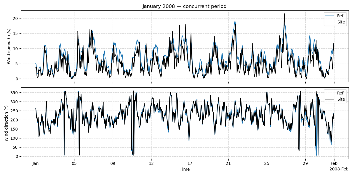
Concurrent Period Time Series

fig, (ax_ws, ax_wd) = plt.subplots(2, 1, figsize=(12, 6), sharex=True)
for ds, color, label in [(ref_st, "C0", "Ref"), (tgt_st, "k", "Site")]:
    sl = ds.sel(time="2008-01")
    sl.wind_speed.plot.line(x="time", ax=ax_ws, color=color, label=label)
    sl.wind_direction.plot.line(x="time", ax=ax_wd, color=color, label=label)
ax_ws.set(
    title="January 2008 — concurrent period", xlabel="", ylabel="Wind speed (m/s)"
)
ax_wd.set(title="", xlabel="Time", ylabel="Wind direction (°)")
for ax in (ax_ws, ax_wd):
    ax.legend()
    ax.grid(True, linestyle="--", alpha=0.5)
fig.tight_layout()

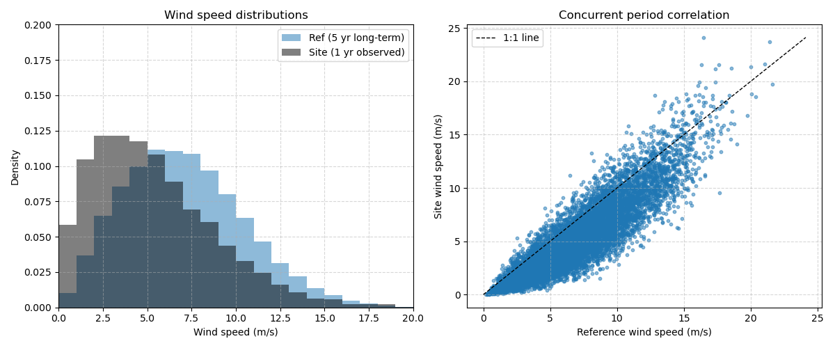
Wind Speed Distributions and Correlation

bins_ws = np.linspace(0.0, 30.0, 31)

fig, (ax1, ax2) = plt.subplots(1, 2, figsize=(12, 5))
kw = dict(bins=bins_ws, density=True, alpha=0.5)
ax1.hist(
    ref_lt.wind_speed.values.flatten(), **kw, color="C0", label="Ref (5 yr long-term)"
)
ax1.hist(
    tgt_st.wind_speed.values.flatten(), **kw, color="k", label="Site (1 yr observed)"
)
ax1.set(
    xlabel="Wind speed (m/s)",
    ylabel="Density",
    title="Wind speed distributions",
    xlim=(0, 20),
    ylim=(0, 0.2),
)
ax1.legend()
ax1.grid(True, linestyle="--", alpha=0.5)

ws_max = max(ref_st.wind_speed.values.max(), tgt_st.wind_speed.values.max())
ax2.scatter(
    ref_st.wind_speed.values.flatten(),
    tgt_st.wind_speed.values.flatten(),
    alpha=0.5,
    color="C0",
    s=10,
)
ax2.plot([0, ws_max], [0, ws_max], "k--", linewidth=1, label="1:1 line")
ax2.set(
    xlabel="Reference wind speed (m/s)",
    ylabel="Site wind speed (m/s)",
    title="Concurrent period correlation",
)
ax2.legend()
ax2.grid(True, linestyle="--", alpha=0.5)
fig.tight_layout()

Fit MCP Models

Both LinRegMCP (ordinary least squares) and VarRatMCP (variance ratio regression) fit one independent regression model per wind direction sector.

linreg = LinRegMCP(n_sectors=12)
linreg.fit(ref_st, tgt_st)

varrat = VarRatMCP(n_sectors=12)
varrat.fit(ref_st, tgt_st)

<windkit.ltc.mcp.VarRatMCP object at 0x7254cb6242f0>

Predict Long-Term Wind Climate

Apply the fitted models to the full 5-year reference to produce a long-term corrected time series at the site location.

predict() returns the deterministic regression-line prediction (conditional mean). predict_with_noise() adds Gaussian noise sampled from the per-sector residual standard deviation, recovering realistic variance in the predicted distribution.

pred_lt_linreg = linreg.predict(ref_lt)
pred_lt_linreg_noisy = linreg.predict_with_noise(ref_lt, seed=42)
pred_lt_varrat = varrat.predict(ref_lt)

Evaluate Model Performance

Use calc_scores() to evaluate how well each model reconstructs the site wind speeds over the concurrent period.

pred_st_linreg = linreg.predict(ref_st)
pred_st_linreg_noisy = linreg.predict_with_noise(ref_st, seed=42)
pred_st_varrat = varrat.predict(ref_st)

scores_baseline = calc_scores(tgt_st, ref_st, name="Baseline", period="Concurrent")
scores_linreg = calc_scores(tgt_st, pred_st_linreg, name="LinReg", period="Concurrent")
scores_linreg_noisy = calc_scores(
    tgt_st, pred_st_linreg_noisy, name="LinReg+noise", period="Concurrent"
)
scores_varrat = calc_scores(tgt_st, pred_st_varrat, name="VarRat", period="Concurrent")

print("BASELINE\n", scores_baseline.to_string(index=False), "\n")
print("LINREG (deterministic)\n", scores_linreg.to_string(index=False), "\n")
print("LINREG (with noise)\n", scores_linreg_noisy.to_string(index=False), "\n")
print("VARRAT\n", scores_varrat.to_string(index=False), "\n")

BASELINE
     Name     Period    Metric     Score
Baseline Concurrent       R^2  0.539602
Baseline Concurrent      RMSE  2.359109
Baseline Concurrent Mean bias -1.721997
Baseline Concurrent       EMD  1.731977

LINREG (deterministic)
   Name     Period    Metric    Score
LinReg Concurrent       R^2 0.795978
LinReg Concurrent      RMSE 1.570435
LinReg Concurrent Mean bias 0.000000
LinReg Concurrent       EMD 0.383193

LINREG (with noise)
         Name     Period    Metric     Score
LinReg+noise Concurrent       R^2  0.614580
LinReg+noise Concurrent      RMSE  2.158481
LinReg+noise Concurrent Mean bias -0.033881
LinReg+noise Concurrent       EMD  0.298426

VARRAT
   Name     Period    Metric    Score
VarRat Concurrent       R^2 0.784246
VarRat Concurrent      RMSE 1.614956
VarRat Concurrent Mean bias 0.000000
VarRat Concurrent       EMD 0.327976

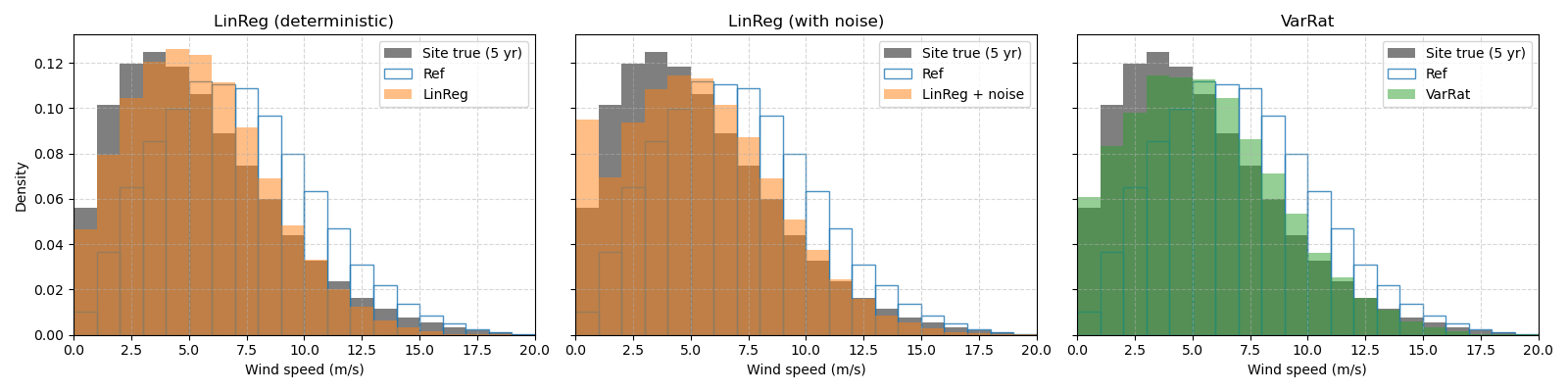
Compare Long-Term Distributions

The deterministic LinReg prediction lies on the regression line and compresses variance — the distribution is too narrow, clipping the high-wind tail. Adding noise via predict_with_noise() recovers the spread by sampling from the per-sector residual distribution. VarRatMCP recovers variance by construction instead: its per-sector slope is set to std(y) / std(x), so the predicted standard deviation matches the target directly without any stochastic sampling.

ws_true = tgt_lt.wind_speed.values.flatten()
ws_ref = ref_lt.wind_speed.values.flatten()
ws_linreg = pred_lt_linreg.wind_speed.values.flatten()
ws_linreg_noisy = pred_lt_linreg_noisy.wind_speed.values.flatten()
ws_varrat = pred_lt_varrat.wind_speed.values.flatten()

kw_true = dict(
    bins=bins_ws, density=True, color="k", alpha=0.5, label="Site true (5 yr)"
)
fig, (ax1, ax2, ax3) = plt.subplots(1, 3, figsize=(16, 4), sharey=True)

ax1.hist(ws_true, **kw_true)
ax1.hist(
    ws_ref,
    bins=bins_ws,
    density=True,
    facecolor="none",
    edgecolor="C0",
    lw=1.0,
    alpha=0.8,
    label="Ref",
)
ax1.hist(ws_linreg, bins=bins_ws, density=True, color="C1", alpha=0.5, label="LinReg")
ax1.set(
    xlabel="Wind speed (m/s)",
    ylabel="Density",
    title="LinReg (deterministic)",
    xlim=(0, 20),
)
ax1.legend()
ax1.grid(True, linestyle="--", alpha=0.5)

ax2.hist(ws_true, **kw_true)
ax2.hist(
    ws_ref,
    bins=bins_ws,
    density=True,
    facecolor="none",
    edgecolor="C0",
    lw=1.0,
    alpha=0.8,
    label="Ref",
)
ax2.hist(
    ws_linreg_noisy,
    bins=bins_ws,
    density=True,
    color="C1",
    alpha=0.5,
    label="LinReg + noise",
)
ax2.set(xlabel="Wind speed (m/s)", title="LinReg (with noise)", xlim=(0, 20))
ax2.legend()
ax2.grid(True, linestyle="--", alpha=0.5)

ax3.hist(ws_true, **kw_true)
ax3.hist(
    ws_ref,
    bins=bins_ws,
    density=True,
    facecolor="none",
    edgecolor="C0",
    lw=1.0,
    alpha=0.8,
    label="Ref",
)
ax3.hist(ws_varrat, bins=bins_ws, density=True, color="C2", alpha=0.5, label="VarRat")
ax3.set(xlabel="Wind speed (m/s)", title="VarRat", xlim=(0, 20))
ax3.legend()
ax3.grid(True, linestyle="--", alpha=0.5)

fig.tight_layout()

Variance Recovery

The standard deviation of the predicted wind speeds shows how deterministic LinReg compresses variance, while predict_with_noise and VarRat both recover the spread.

print(f"Site true std:           {np.std(ws_true):.3f} m/s")
print(f"LinReg (deterministic):  {np.std(ws_linreg):.3f} m/s")
print(f"LinReg (with noise):     {np.std(ws_linreg_noisy):.3f} m/s")
print(f"VarRat:                  {np.std(ws_varrat):.3f} m/s")

Site true std:           3.447 m/s
LinReg (deterministic):  3.040 m/s
LinReg (with noise):     3.340 m/s
VarRat:                  3.412 m/s