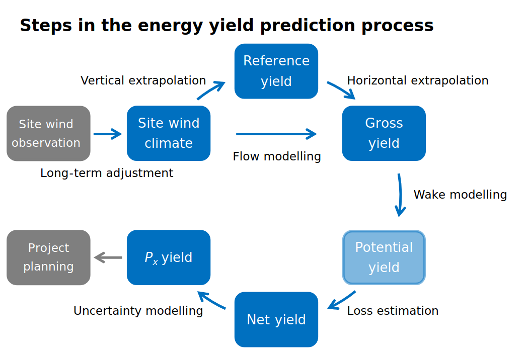
Calculate AEP#
PyWAsP can estimate the Annual Energy Production (AEP) of wind turbines.
This includes estimating the gross and potential AEP (as shown in the workflow below), as well as support for estimating net AEP (P50) and P90.
We will start by importing the necessary libraries and some test data from the Serra Santa Luzia site.
In [1]: import numpy as np

In [2]: import pandas as pd

In [3]: import xarray as xr

In [4]: import matplotlib.pyplot as plt

In [5]: import windkit as wk

In [6]: import pywasp as pw
In [7]: tutorial_data = wk.load_tutorial_data("serra_santa_luzia")

In [8]: bwc = tutorial_data.bwc

In [9]: elev_map = tutorial_data.elev

In [10]: rgh_map = tutorial_data.rgh

In [11]: topo_map = pw.wasp.TopographyMap(elev_map, rgh_map)

In [12]: gwc = pw.wasp.generalize(bwc, topo_map)
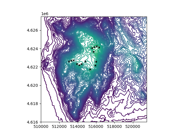
We have used this site in the WAsP Flow Model page, but here we will
go further and include some turbines. Their locations are stored in a .csv file,
so we will create an xarray.Dataset to hold their spatial information: x, y, and hub height.
We can plot their locations together with the elevation map to get an idea of where they are located:
In [13]: wtg_locs = pd.read_csv('./source/tutorials/data/turbine_positions.csv')

In [14]: output_locs =  wk.spatial.create_point(
   ....:     wtg_locs.Easting.values,
   ....:     wtg_locs.Northing.values,
   ....:     wtg_locs['Hub height'].values,
   ....:     crs="EPSG:32629"
   ....: )
   ....:

In [15]: fig, ax = plt.subplots()

In [16]: ax.set(xlim=(510000, 521500), ylim=(4616000, 4627500))
Out[16]: [(510000.0, 521500.0), (4616000.0, 4627500.0)]

In [17]: elev_map.plot("elev", ax=ax);

In [18]: ax.scatter(
   ....:     output_locs.west_east.values,
   ....:     output_locs.south_north.values,
   ....:     c="k",
   ....:     marker="x",
   ....:     s=15,
   ....:     zorder=2,
   ....: );
   ....:
To estimate the AEP, we will first estimate the wind climate at the hub height of each turbine:
In [19]: wwc = pw.wasp.predict_wwc(bwc, topo_map, output_locs)

In [20]: print(wwc)
<xarray.Dataset> Size: 3kB
Dimensions:        (point: 15, sector: 12)
Coordinates:
    height         (point) int64 120B 50 50 50 50 50 50 50 ... 50 50 50 50 50 50
    south_north    (point) int64 120B 4622313 4622199 ... 4624252 4624142
    west_east      (point) int64 120B 513914 514161 514425 ... 516060 516295
  * sector         (sector) float64 96B 0.0 30.0 60.0 90.0 ... 270.0 300.0 330.0
    sector_ceil    (sector) float64 96B 15.0 45.0 75.0 ... 285.0 315.0 345.0
    sector_floor   (sector) float64 96B 345.0 15.0 45.0 ... 255.0 285.0 315.0
    crs            int8 1B 0
Dimensions without coordinates: point
Data variables:
    A              (sector, point) float32 720B 7.432 7.405 ... 7.716 8.268
    k              (sector, point) float32 720B 2.025 2.033 ... 2.131 2.127
    wdfreq         (sector, point) float32 720B 0.06444 0.06484 ... 0.07929
    site_elev      (point) float32 60B 459.7 460.0 460.0 ... 520.0 520.0 520.0
    air_density    (point) float32 60B 1.163 1.163 1.163 ... 1.156 1.156 1.156
    wspd           (point) float32 60B 7.485 7.307 7.027 ... 7.595 7.861 8.145
    power_density  (point) float32 60B 422.7 392.7 347.5 ... 433.9 489.4 540.2
Attributes:
    Conventions:      CF-1.8
    history:          2026-01-29T14:39:18+00:00:\twindkit==2.0.0\t"point")\n2...
    title:            WAsP site effects
    Package name:     windkit
    Package version:  2.0.0
    Creation date:    2026-01-29T14:39:19+00:00
    Object type:      Met fields
    author:           Neil Davis
    author_email:     neda@dtu.dk
    institution:      DTU Wind and Energy Systems
Gross AEP#
Before we estimate the AEP, we need to get a Wind Turbine Generator (wtg) corresponding to the turbine models used.
We use windkit.read_wtg() to read the .wtg file.
In [21]: wtg = wk.read_wtg("./source/tutorials/data/Bonus_1_MW.wtg")

In [22]: print(wtg)
<xarray.Dataset> Size: 704B
Dimensions:                        (mode: 1, wind_speed: 22)
Coordinates:
  * mode                           (mode) int64 8B 0
  * wind_speed                     (wind_speed) float64 176B 4.0 5.0 ... 25.0
Data variables:
    power_output                   (mode, wind_speed) float64 176B 2.41e+04 ....
    thrust_coefficient             (mode, wind_speed) float64 176B 0.915 ... ...
    air_density                    (mode) float64 8B 1.225
    stationary_thrust_coefficient  (mode) float64 8B 0.161
    wind_speed_cutin               (mode) float64 8B 4.0
    wind_speed_cutout              (mode) float64 8B 25.0
    rated_power                    (mode) float64 8B 1e+06
    name                           <U10 40B 'Bonus 1 MW'
    manufacturer                   <U16 64B 'Bonus Energy A/S'
    rotor_diameter                 float64 8B 54.2
    hub_height                     float64 8B 50.0
    regulation_type                int64 8B 2
Attributes:
    Conventions:      CF-1.8
    Package name:     windkit
    Package version:  2.0.0
    Creation date:    2026-01-29T14:39:19+00:00
    author:           Neil Davis
    author_email:     neda@dtu.dk
    institution:      DTU Wind and Energy Systems
The wtg holds power and thrust curves for a number of wind speeds and operational modes (in this case, just one operational mode).
The wtg also contains extra information, which can be either mode-specific, such as air_density, cut_in_wind_speed, cut_out_wind_speed, rated_wind_speed,
or dimensionless, such as name, manufacturer, rotor_diameter, hub_height, and regulation_type.
We can now estimate the gross AEP using pywasp.gross_aep(), passing at least a wwc and a wtg object:
In [23]: aep = pw.gross_aep(wwc, wtg)

In [24]: print(aep)
<xarray.Dataset> Size: 1kB
Dimensions:           (point: 15, sector: 12)
Coordinates:
    height            (point) int64 120B 50 50 50 50 50 50 ... 50 50 50 50 50 50
    south_north       (point) int64 120B 4622313 4622199 ... 4624252 4624142
    west_east         (point) int64 120B 513914 514161 514425 ... 516060 516295
  * sector            (sector) float64 96B 0.0 30.0 60.0 ... 270.0 300.0 330.0
    sector_ceil       (sector) float64 96B 15.0 45.0 75.0 ... 285.0 315.0 345.0
    sector_floor      (sector) float64 96B 345.0 15.0 45.0 ... 255.0 285.0 315.0
    crs               int8 1B 0
Dimensions without coordinates: point
Data variables:
    gross_aep         (point) float32 60B 2.835 2.7 2.487 ... 2.907 3.096 3.31
    gross_aep_sector  (point, sector) float32 720B 0.143 0.08603 ... 0.2167
Attributes:
    Conventions:      CF-1.8
    history:          2026-01-29T14:39:18+00:00:\twindkit==2.0.0\t"point")\n2...
    title:            WAsP site effects
    Package name:     windkit
    Package version:  2.0.0
    Creation date:    2026-01-29T14:39:19+00:00
    Object type:      Anual Energy Production
    author:           Neil Davis
    author_email:     neda@dtu.dk
    institution:      DTU Wind and Energy Systems

In [25]: print(aep["gross_aep"].values.sum(), "GWh")
42.201473 GWh
Passing simply a wwc and a wtg works well when your climate is predicted for exactly the hub heights and locations
of the same turbine type for which you want to estimate AEP.
However, it may be the case that a project has different turbines across the same wind farm.
To handle this, a more flexible approach is needed. Instead of a single wtg, a dictionary of wtg’s and a dataset of
turbine locations, heights, turbine ids, group ids, and wtg keys that
map to the wtg’s in the dictionary should be passed. In the example below, we show how to do this and how to make use of the extra keyword arguments in the pywasp.gross_aep() function.
In [26]: v90_wtg = wk.read_wtg("./source/tutorials/data/V90-3.0MW_VCRS_60hz.wtg")
In [27]: wtg_dict = {"Bonus_1_MW":wtg, "V90-3.0MW_VCRS_60hz":v90_wtg }
In [28]: output_locs_updated = output_locs.copy(deep=True)
In [29]: output_locs_updated["height"].loc[dict(point=range(10, 15))] = 80
In [30]: wwc_updated = pw.wasp.predict_wwc(bwc, topo_map, output_locs_updated)
In [31]: wind_turbines = wk.create_wind_turbines_from_arrays(
....: west_east=output_locs_updated.west_east.values,
....: south_north=output_locs_updated.south_north.values,
....: height=output_locs_updated.height.values,
....: wtg_keys=["Bonus_1_MW"] * 10 + ["V90-3.0MW_VCRS_60hz"] * 5,
....: group_ids=np.zeros(15),
....: turbine_ids=np.arange(15),
....: )
....:
In [32]: aep_updated = pw.gross_aep(
....: wwc_updated,
....: wtg_dict,
....: wind_turbines,
....: use_sectors=True,
....: air_density_correction="infer",
....: air_density=None)
....:
In [33]: print(aep_updated)
<xarray.Dataset> Size: 1kB
Dimensions: (point: 15, sector: 12)
Coordinates:
height (point) int64 120B 50 50 50 50 50 50 ... 50 80 80 80 80 80
south_north (point) int64 120B 4622313 4622199 ... 4624252 4624142
west_east (point) int64 120B 513914 514161 514425 ... 516060 516295
* sector (sector) float64 96B 0.0 30.0 60.0 ... 270.0 300.0 330.0
sector_ceil (sector) float64 96B 15.0 45.0 75.0 ... 285.0 315.0 345.0
sector_floor (sector) float64 96B 345.0 15.0 45.0 ... 255.0 285.0 315.0
crs int8 1B 0
Dimensions without coordinates: point
Data variables:
gross_aep (point) float32 60B 2.835 2.7 2.487 ... 9.035 9.445 9.883
gross_aep_sector (point, sector) float32 720B 0.143 0.08603 ... 0.6439
Attributes:
Conventions: CF-1.8
history: 2026-01-29T14:39:18+00:00:\twindkit==2.0.0\t"point")\n2...
title: WAsP site effects
Package name: windkit
Package version: 2.0.0
Creation date: 2026-01-29T14:39:20+00:00
Object type: Anual Energy Production
author: Neil Davis
author_email: neda@dtu.dk
institution: DTU Wind and Energy Systems
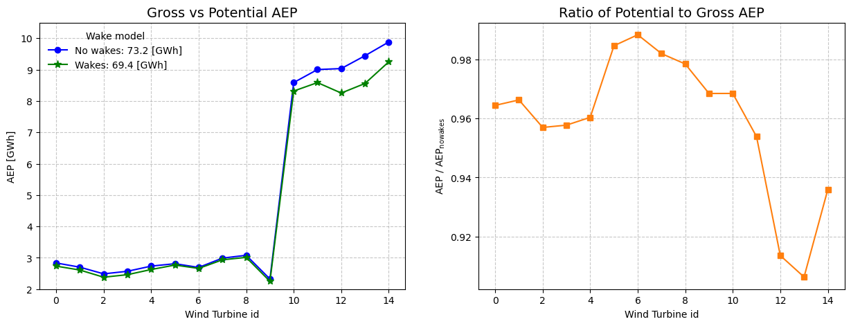
In [34]: print(aep_updated["gross_aep"].values.sum(), "GWh")
73.174034 GWh
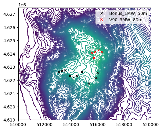
In the example above, we introduce an additional turbine type, the “V90-3.0MW_VCRS_60hz”, which has a different hub height compared to the existing “Bonus_1_MW” turbines. Specifically, we effectively replace the last five turbines with the new turbine model.
Therefore, we must first predict the wind climate at the correct hub heights. Initially, the output locations assume a hub height of 50 m for the first ten turbines (Bonus_1_MW). However, since the newly introduced turbines operate at 80 m, we update the output locations accordingly to reflect this difference.
Once the wind climate has been downscaled to the revised hub heights,
we proceed with creating a wind turbines dataset that correctly maps turbine types to their respective locations.
This dataset, represented by the wind_turbines object, contains:
- turbine locations
- hub heights
- wtg keys (to name the turbine model)
- group ids (to categorize the different groups of turbines within a wind farm)
- turbine ids (unique integer identifiers for each turbine)
When working with multiple turbine types, it is essential to
make sure that the wtg_keys name matches the dictionary key passed in the wtg_dict object.
Notice that the last 5 turbines in the wind_turbines object have a value of “V90-3.0MW_VCRS_60hz” in the wtg_keys attribute.
There is no limit to the number of turbine models that can be used in this approach.
Additionally, turbine IDs must be unique integers, typically assigned based on the order of west-east and south-north locations for consistency.
Moreover, extra keyword arguments in the pywasp.gross_aep() function can be used to further customize the AEP estimation.
In this example, we use the default values:
use_sectors: Defaults toTrueto use sector-wise “A” and “k”. If set toFalse, “A_combined” and “k_combined” are used for the AEP calculation.
air_density_correction: Defaults to"infer", which means that air density is inferred from the wind climate and thewtgpower curve gets corrected to account for site-specific air density. If set to"none", no correction is applied to the power curve, and the default air density mode is used to calculate produced power.
air_density: Can be passed with a value to override the inferred air density.
Potential AEP#
To add wind farm effects, such as wakes and blockage, to the AEP estimation and obtain the
“potential AEP”, PyWAsP integrates with PyWake. PyWAsP defines a number
of named wind farm models, see pywasp.potential_aep(), including “PARK2_onshore” and “PARK2_offshore”,
that are identical to the wake model in the WAsP GUI. Here we will use the onshore version:
In [35]: aep_wakes = pw.potential_aep(wwc,
   ....:     wtg,
   ....:     wind_farm_model="PARK2_onshore",
   ....:     turbulence_intensity=0.0
   ....: )
   ....:

In [36]: print(aep_wakes)
<xarray.Dataset> Size: 12kB
Dimensions:                          (sector: 12, point: 15)
Coordinates:
  * sector                           (sector) float64 96B 0.0 30.0 ... 330.0
  * point                            (point) int64 120B 0 1 2 3 ... 11 12 13 14
    height                           (point) int64 120B 50 50 50 50 ... 50 50 50
    south_north                      (point) int64 120B 4622313 ... 4624142
    west_east                        (point) int64 120B 513914 514161 ... 516295
    crs                              int8 1B 0
    mode                             int64 8B 0
Data variables: (12/15)
    potential_aep_sector             (point, sector) float64 1kB 0.143 ... 0....
    gross_aep_sector                 (point, sector) float64 1kB 0.144 ... 0....
    potential_aep_deficit_sector     (point, sector) float64 1kB 0.00666 ... ...
    wspd_sector                      (point, sector) float64 1kB 6.585 ... 7.323
    wspd_eff_sector                  (point, sector) float64 1kB 6.585 ... 7.323
    wspd_deficit_sector              (point, sector) float64 1kB 0.0 ... 0.0
    ...                               ...
    gross_aep                        (point) float64 120B 2.846 2.71 ... 3.317
    potential_aep_deficit            (point) float64 120B 0.04798 ... 0.03901
    wspd                             (point) float64 120B 7.485 7.307 ... 8.145
    wspd_eff                         (point) float64 120B 7.359 7.19 ... 8.0
    wspd_deficit                     (point) float64 120B 0.01847 ... 0.01782
    turbulence_intensity_eff         (point) float64 120B 0.0 0.0 ... 0.0 0.0
Attributes:
    Conventions:      CF-1.8
    history:          2026-01-29T14:39:18+00:00:\twindkit==2.0.0\t"point")\n2...
    title:            WAsP site effects
    Package name:     windkit
    Package version:  2.0.0
    Creation date:    2026-01-29T14:39:20+00:00
    Object type:      Anual Energy Production
    author:           Neil Davis
    author_email:     neda@dtu.dk
    institution:      DTU Wind and Energy Systems

In [37]: print(aep_wakes["potential_aep"].values.sum(), "GWh")
40.83236248207012 GWh
We can also calculate the potential AEP for the updated turbine models and locations:
In [38]: aep_wakes_updated = pw.potential_aep(
   ....:     wwc_updated,
   ....:     wtg_dict,
   ....:     wind_turbines,
   ....:     wind_farm_model="PARK2_onshore",
   ....:     turbulence_intensity=0.0,
   ....:     shear = None,
   ....:     air_density_correction="infer"
   ....: )
   ....:

In [39]: print(aep_wakes_updated)
<xarray.Dataset> Size: 12kB
Dimensions:                          (sector: 12, point: 15)
Coordinates:
  * sector                           (sector) float64 96B 0.0 30.0 ... 330.0
  * point                            (point) int64 120B 0 1 2 3 ... 11 12 13 14
    height                           (point) int64 120B 50 50 50 50 ... 80 80 80
    south_north                      (point) int64 120B 4622313 ... 4624142
    west_east                        (point) int64 120B 513914 514161 ... 516295
    crs                              int8 1B 0
    mode                             int64 8B 0
Data variables: (12/15)
    potential_aep_sector             (point, sector) float64 1kB 0.143 ... 0....
    gross_aep_sector                 (point, sector) float64 1kB 0.144 ... 0....
    potential_aep_deficit_sector     (point, sector) float64 1kB 0.006655 ......
    wspd_sector                      (point, sector) float64 1kB 6.585 ... 7.457
    wspd_eff_sector                  (point, sector) float64 1kB 6.585 ... 7.443
    wspd_deficit_sector              (point, sector) float64 1kB 0.0 ... 0.00...
    ...                               ...
    gross_aep                        (point) float64 120B 2.846 2.711 ... 9.897
    potential_aep_deficit            (point) float64 120B 0.05001 ... 0.06625
    wspd                             (point) float64 120B 7.485 7.307 ... 8.31
    wspd_eff                         (point) float64 120B 7.355 7.186 ... 8.046
    wspd_deficit                     (point) float64 120B 0.01912 ... 0.03158
    turbulence_intensity_eff         (point) float64 120B 0.0 0.0 ... 0.0 0.0
Attributes:
    Conventions:      CF-1.8
    history:          2026-01-29T14:39:18+00:00:\twindkit==2.0.0\t"point")\n2...
    title:            WAsP site effects
    Package name:     windkit
    Package version:  2.0.0
    Creation date:    2026-01-29T14:39:20+00:00
    Object type:      Anual Energy Production
    author:           Neil Davis
    author_email:     neda@dtu.dk
    institution:      DTU Wind and Energy Systems

In [40]: print(aep_wakes_updated["potential_aep"].values.sum(), "GWh")
69.32647698974341 GWh
Notice that pywasp.potential_aep() needs to be passed with extra keyword arguments turbulence_intensity (mandatory) and shear (optional).
Moreover, the same characteristics regarding the air density correction arguments in pywasp.gross_aep() function apply for pywasp.potential_aep(),
where again, there is no limit to the number of turbine models that can be used.
From the complex case above we can see how, even though, we achieve higher power with the larger turbines, these also generate a considerable amount of wake losses.
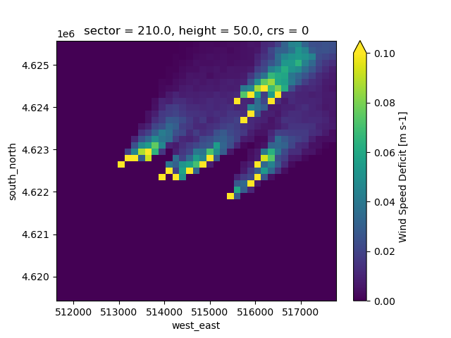
Wind farm flow map#
To map an area around a wind farm, PyWAsP has pywasp.wind_farm_flow_map(), which
takes a resource grid as input and enriches it with wind farm variables including
effects of nearby turbines. This function gives a detailed visualization of the wind farm effects.
Currently, the use of different turbine models populating the wind farm is not supported.
Thus, the example below corresponds to the case where the wind farm is fully populated with the “Bonus_1_MW” turbine.
In [41]: output_grid = wk.spatial.create_dataset(
   ....:     np.linspace(511700.0, 517700.0, 31),
   ....:     np.linspace(4619500.0, 4625500.0, 31),
   ....:     [50.0],
   ....:     crs="EPSG:32629",
   ....: )
   ....:

In [42]: wwc_grid = pw.wasp.downscale(gwc, topo_map, output_grid, interp_method="nearest")

In [43]: wind_turbines = wk.create_wind_turbines_from_arrays(
   ....:     west_east=output_locs.west_east.values,
   ....:     south_north=output_locs.south_north.values,
   ....:     height=output_locs.height.values,
   ....:     wtg_keys=["Bonus 1 MW"]*15,
   ....:     group_ids=np.zeros(15, dtype=int),
   ....:     turbine_ids=np.arange(15, dtype=int),
   ....: )
   ....:

In [44]: flow_map = pw.wind_farm_flow_map(
   ....:     wwc_grid,
   ....:     wtg,
   ....:     wind_turbines,
   ....:     output_grid,
   ....:     wind_farm_model="PARK2_onshore",
   ....:     turbulence_intensity=0.0
   ....: )
   ....:

In [45]: print(flow_map)
<xarray.Dataset> Size: 746kB
Dimensions:                          (sector: 12, height: 1, south_north: 31,
                                      west_east: 31)
Coordinates:
  * sector                           (sector) float64 96B 0.0 30.0 ... 330.0
  * height                           (height) float64 8B 50.0
  * south_north                      (south_north) float64 248B 4.62e+06 ... ...
  * west_east                        (west_east) float64 248B 5.117e+05 ... 5...
    crs                              int8 1B 0
    mode                             int64 8B 0
Data variables: (12/15)
    potential_aep_sector             (height, south_north, west_east, sector) float64 92kB ...
    gross_aep_sector                 (height, south_north, west_east, sector) float64 92kB ...
    potential_aep_deficit_sector     (height, south_north, west_east, sector) float64 92kB ...
    wspd_sector                      (height, south_north, west_east, sector) float64 92kB ...
    wspd_eff_sector                  (height, south_north, west_east, sector) float64 92kB ...
    wspd_deficit_sector              (height, south_north, west_east, sector) float64 92kB ...
    ...                               ...
    gross_aep                        (height, south_north, west_east) float64 8kB ...
    potential_aep_deficit            (height, south_north, west_east) float64 8kB ...
    wspd                             (height, south_north, west_east) float64 8kB ...
    wspd_eff                         (height, south_north, west_east) float64 8kB ...
    wspd_deficit                     (height, south_north, west_east) float64 8kB ...
    turbulence_intensity_eff         (height, south_north, west_east) float64 8kB ...
Attributes:
    Conventions:      CF-1.8
    history:          2026-01-29T14:39:20+00:00:\twindkit==2.0.0\twk.spatial....
    Package name:     windkit
    Package version:  2.0.0
    Creation date:    2026-01-29T14:39:25+00:00
    Object type:      Wind Farm Flow Map
    author:           Neil Davis
    author_email:     neda@dtu.dk
    institution:      DTU Wind and Energy Systems
    title:            WAsP site effects
Notice that in wind_farm_flow_map(), the first argument, namely the wind climate, is a gridded wind climate.
This is because we need to wrap the wind turbines of the wind farm in a large enough cuboid to capture the upstream and downstream effects.
By modifying the output_grid x and y linespace, a finer or coarser resolution in the grid can be obtained.
Remember to set the cuboid height to the hub height of the turbines, in this case 50 m.
Additionally, the wind_turbines object is also mandatory to be passed, as the function needs to know the exact location of the turbines within the cuboid.
The pywasp.wind_farm_flow_map() function outputs an updated xarray.Dataset with the wind speed and AEP deficits. We can later use these to generate plots,
for example, the wind speed deficit at one directional sector to visualize the wake effects:
In [46]: flow_map["wspd_deficit_sector"].sel(sector=210).plot(vmax=0.1)
Net AEP#
To add other losses after wake effects towards the AEP estimation and obtain the “net AEP”, we can do so by importing a loss table with the windkit function wk.get_loss_table().
For now, only one table is available, that is a “dtu-default” loss table, which can be modified and personalized by the user.
PyWAsP Tutorial 6, shows an extended use case of the loss module.
Once the loss table is imported, the pywasp.net_aep() function can be used to estimate the net AEP.
In [47]: loss_table = wk.get_loss_table()

In [48]: print(wk.loss_table_summary(loss_table))
Loss Summary:
Total value of losses for Availability: 1.5 %
Total value of losses for Curtailments: 0.5 %
Total value of losses for Electrical: 0.7 %
Total value of losses for Environmental: 0.35 %
Total value of losses for Operational_strategies: 0.5 %
Total value of losses for Turbine_performance: 1.0 %
Total value of all losses: 4.550000000000001 %
None

In [49]: net_aep = pw.net_aep(loss_table, aep_wakes)

In [50]: print(net_aep["net_aep"].sum().values, "GWh")
38.97448998913593 GWh
Px yield#
The P90 yield, that is the AEP bankable number with 90% probability of being achieved or surpassed, can be estimated in a similar way, but has some extra steps involved in the process. For a more detailed overview, please refer to Tutorial 6 to see the full process and usage of these functions.
In this simplified approach, first an uncertainty table must be loaded, and if desired, personalized.
Next, we must estimate the sensitivity factor, which tells the model how sensitive the AEP is to wind speed. For this, the pywasp.estimate_sensitivity_factor() function is used.
Note that this function requires the wind climate, the wind turbine generator, and a wind perturbation factor.
Ideally, for the wind_perturbation_factor, the wind-speed dimensional standard deviation should be passed. This can be retrieved using the windkit function windkit.total_uncertainty() and later multiplying by the local wind speed.
Finally, the P90 yield is estimated with the pywasp.px_aep() function, although one could also estimate any other AEP associated with a probability, such as P50, P75, etc., by changing the percentile argument.
In [51]: uncertainty_table = wk.get_uncertainty_table()

In [52]: Uave = wk.mean_wind_speed(wwc, bysector=False)

In [53]: _, wind_uncertainty, _ = wk.total_uncertainty(uncertainty_table)

In [54]: sigma_wind_dimensional =  wind_uncertainty/100 * Uave.values.mean()

In [55]: print(sigma_wind_dimensional, "m/s")
0.38308626181941 m/s

In [56]: sf = pw.estimate_sensitivity_factor(wwc, wtg, wind_perturbation_factor=sigma_wind_dimensional)

In [57]: print("The sensitivity factor is:", sf)
The sensitivity factor is: 1.8076315253508868

In [58]: p90 = pw.px_aep(uncertainty_table, net_aep, sensitivity_factor=sf, percentile=90)

In [59]: print("The P90 is:", p90["P_90_aep"].values.sum(), "GWh")
The P90 is: 33.9132490394319 GWh
PyWake integration in PyWAsP#
PyWAsP can use PyWake wind farm models to estimate the potential AEP. This is done by passing the name of the PyWake wind farm model to the pywasp.potential_aep() and pywasp.wind_farm_flow_map() functions.
To ensure stability and consistency of PyWAsP, the PyWake versions for each PyWAsP release is pinned to a specific version of PyWake. When installing PyWAsP via mamba, the correct version of PyWake is installed automatically.
We periodically update the pinned version of PyWake to the latest version that is compatible with PyWAsP.
Using custom PyWake wind farm models#
Instead of using a named wind farm model, it is possible to construct a
PyWake wind farm model manually, using functools.partial(), and use it for adding wind farm effects in PyWAsP:
In [60]: from functools import partial

In [61]: import py_wake

In [62]: wind_farm_model = partial(
   ....:     py_wake.wind_farm_models.engineering_models.All2AllIterative,
   ....:     wake_deficitModel=py_wake.deficit_models.noj.NOJLocalDeficit(
   ....:         a=[0, 0.06],
   ....:         ct2a=py_wake.deficit_models.utils.ct2a_mom1d,
   ....:         use_effective_ws=True,
   ....:         use_effective_ti=False,
   ....:         rotorAvgModel=py_wake.rotor_avg_models.AreaOverlapAvgModel(),
   ....:     ),
   ....:     superpositionModel=py_wake.superposition_models.LinearSum(),
   ....:     blockage_deficitModel=py_wake.deficit_models.Rathmann(),
   ....:     deflectionModel=None,
   ....:     turbulenceModel=None,
   ....: )
   ....:

In [63]: aep_wakes_personalized_model = pw.potential_aep(
   ....:     wwc,
   ....:     wtg,
   ....:     wind_farm_model=wind_farm_model,
   ....:     turbulence_intensity=0.0
   ....: )
   ....:

In [64]: print(aep_wakes_personalized_model)
<xarray.Dataset> Size: 12kB
Dimensions:                          (sector: 12, point: 15)
Coordinates:
  * sector                           (sector) float64 96B 0.0 30.0 ... 330.0
  * point                            (point) int64 120B 0 1 2 3 ... 11 12 13 14
    height                           (point) int64 120B 50 50 50 50 ... 50 50 50
    south_north                      (point) int64 120B 4622313 ... 4624142
    west_east                        (point) int64 120B 513914 514161 ... 516295
    crs                              int8 1B 0
    mode                             int64 8B 0
Data variables: (12/15)
    potential_aep_sector             (point, sector) float64 1kB 0.143 ... 0....
    gross_aep_sector                 (point, sector) float64 1kB 0.144 ... 0....
    potential_aep_deficit_sector     (point, sector) float64 1kB 0.006898 ......
    wspd_sector                      (point, sector) float64 1kB 6.585 ... 7.323
    wspd_eff_sector                  (point, sector) float64 1kB 6.584 ... 7.331
    wspd_deficit_sector              (point, sector) float64 1kB 9.693e-05 .....
    ...                               ...
    gross_aep                        (point) float64 120B 2.846 2.71 ... 3.317
    potential_aep_deficit            (point) float64 120B 0.05511 ... 0.04658
    wspd                             (point) float64 120B 7.485 7.307 ... 8.145
    wspd_eff                         (point) float64 120B 7.336 7.161 ... 7.967
    wspd_deficit                     (point) float64 120B 0.02175 ... 0.02185
    turbulence_intensity_eff         (point) float64 120B 0.0 0.0 ... 0.0 0.0
Attributes:
    Conventions:      CF-1.8
    history:          2026-01-29T14:39:18+00:00:\twindkit==2.0.0\t"point")\n2...
    title:            WAsP site effects
    Package name:     windkit
    Package version:  2.0.0
    Creation date:    2026-01-29T14:39:25+00:00
    Object type:      Anual Energy Production
    author:           Neil Davis
    author_email:     neda@dtu.dk
    institution:      DTU Wind and Energy Systems

In [65]: print(aep_wakes_personalized_model["potential_aep"].values.sum(), "GWh")
40.541991759257144 GWh
Calculating AEP including wake effects#
In PyWAsP, the “park” method is used in py_wake.Site.XRSsite.from_pwc() for calculating the speed-up when passing the wind climate to a py_wake site object.
The steps used to calculate the AEP including wake effects are as follows:
Flow cases are defined to ensure all possible/relevant directions and speeds are covered. The wind speed in each flow case is relative to the maximum mean wind speed in the sector.
The wind farm simulation results from py_wake contains the variable two different wind speed variables. One is
WS, which is inhomogeneous background (free) wind speed used to obtain the probability density from the individual sector-wise weibull distributions. Another one is variableWS_eff, which contains the effective wind speed after including wind farm effects.The AEP is determined by finding the effective power curves relative to the background wind speed
P_eff(WS)and performing an integral over wind speed.