WAsP Flow Model#
WAsP includes flow models for horizontal and vertical extrapolation of wind climates. The models includes effects on the flow from terrain inhomogeneity and from the structure of the atmospheric surface layer.
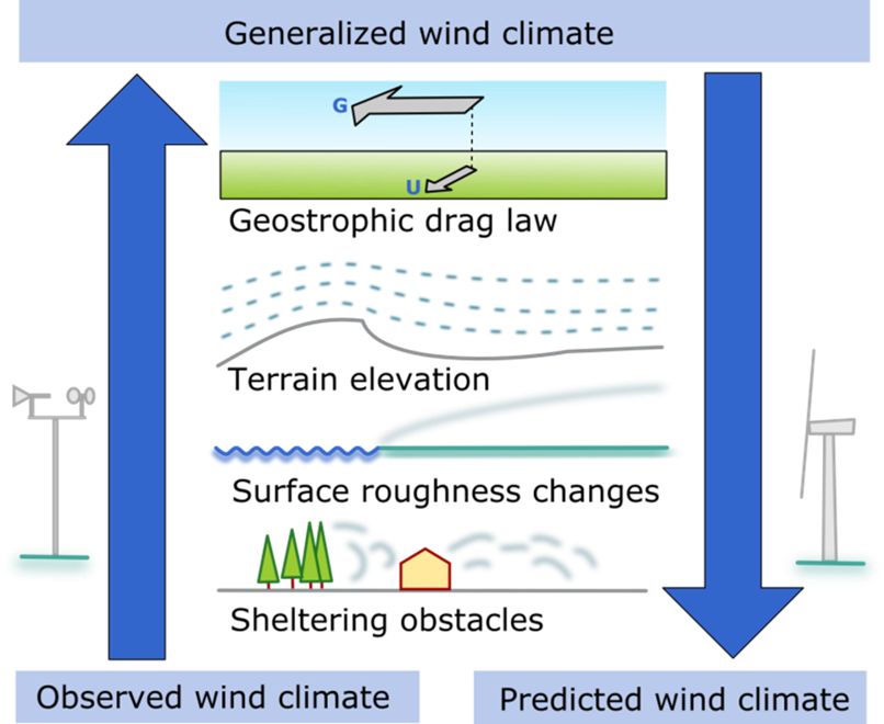
Illustration of the generalization (up arrow) and downscaling (down arrow) which is the key idea of extrapolation of wind climates in WAsP#
- Core to the flow extrapolation in WAsP is the two steps illustrated in the figure above:
Generalization
Downscaling
Generalization is the process of “removing” local terrain and surface layer effects from the observed wind climate and instead “generalizing” the wind climate to a number of “standard” conditions (of surface roughness and height above ground).
Downscaling is the reverse process where local terrain and surface layer effects are “added” to the generalized wind climate to obtain new (weibull) wind climates at desired locations.
A generalized wind climate tries to be representative of a larger area, an observed and predicted wind climate is representative only of a specific location.
PyWAsP makes it possible to perform these two steps individually, or combined into a single call for
when you know the observed wind climate and the desired output locations from the start. Two main
functions exists for such “direct” wind climate extrapolation: predict_wwc() and predict_bwc().
The first, predict_wwc(), is used when you have a binned wind climate and want the results returned
as a weibull wind climate. The second, predict_bwc(), is used when you want a binned wind climate as output.
The last option is useful when you want to preserve a lot of the information in the observed wind climate, by avoiding
the weibull fitting step.
WAsP flow effects and submodels#
WAsP makes corrections to wind climates during both generalization and downscaling. The corrections are based on different effects that are modeled in different WAsP submodels. They include:
Orographic flow effects (BZ model)
Internal boundary layer (IBL model)
Geostrophic drag-law
Atmospheric stability model
The first two components are terrain effects, linear scaling factors that are derived directly from the terrain data. The last two components are climate effects, non-linear effects (in wind speed), that are handled by the WAsP climate model during the generalization and downscaling steps. The main flow effect from roughness are typically not the internal boundary layer effects, but the shift in effective roughness when going from the origin site to the target site. These effects are coming via the geostrophic drag-law, which uses the effective roughnesses for the specific sites and sectors to calculate the effective wind speeds. For more details on the geostrophic drag-law in WAsP, see e.g. the European wind atlas chapter 8.7 and 8.8 <https://backend.orbit.dtu.dk/ws/portalfiles/portal/112135732/European_Wind_Atlas.pdf>_ . The stability model is described in the appendix of this paper <https://link.springer.com/article/10.1007/s10546-023-00803-3>_ .
To illustrate the flow model, we will import pywasp, windkit, and some other commonly used libraries.
In [1]: import numpy as np

In [2]: import xarray as xr

In [3]: import matplotlib.pyplot as plt

In [4]: import windkit as wk

In [5]: import pywasp as pw
We will also use terrain and wind data from the Santa Luzia site.
In [6]: bwc = wk.read_bwc("./source/tutorials/data/SerraSantaLuzia.omwc", crs="EPSG:4326")

In [7]: bwc = wk.spatial.reproject(bwc, to_crs="EPSG:32629")

In [8]: elev_map = wk.read_elevation_map(
   ...:     "source/tutorials/data/SerraSantaLuzia.map",
   ...:     crs="EPSG:32629",
   ...: )
   ...:

In [9]: rgh_map = wk.read_roughness_map(
   ...:     "source/tutorials/data/SerraSantaLuzia.map",
   ...:     crs="EPSG:32629",
   ...: )
   ...:

In [10]: topo_map = pw.wasp.TopographyMap(
   ....:     elev_map,
   ....:     rgh_map
   ....: )
   ....:
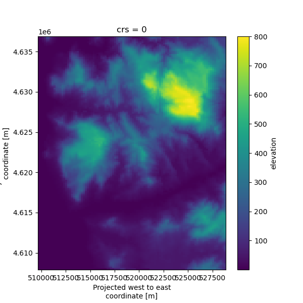
To get a sense of the topography at the site, we will plot the elevation and roughness maps. It easiest to visualize the roughness data as a raster map, because the vector map version is roughness-change lines, which can be hard to detect patterns from. So, we will convert to raster data first, and then plot it. First the elevation:
In [11]: elev_raster = pw.vector_to_raster(elev_map, res=200)

In [12]: elev_raster.plot()
Second, the surface roughness:
In [13]: ax_lc = wk.plot.landcover_map(rgh_map, zorder=0)

In [14]: wk.spatial.ds_to_gdf(bwc).plot(ax=ax_lc, zorder=1, color="black", marker="X", markersize=40)
Out[14]: <Axes: xlabel='Easting (m)', ylabel='Northing (m)'>
or
In [15]: rgh_map.explore("z0")
Out[15]: <folium.folium.Map at 0x782fd3ecacf0>
From the maps we see flat land with low roughness along the western edge covered by ocean. Inland, to the northwest, and to the northeast we see two hills with lower roughness on the top. In the south, low surface roughness and flat elevation reveals a river wedged into the land, stretching from west to east.
Terrain effects#
Now that we have created a TopographyMap and inspected the topography at the site,
let us start modeling terrain effects using the WAsP model. From the topography map, we can
obtain the linearized effects from the terrain model, which includes orographic speed-ups and turnings,
and internal boundary layer speed-ups, due to roughness changes.
First, we will define output locations by using windkit.spatial.create_dataset().
In this case, we define a 41x41x1 cuboid-shaped output grid (1681 total points).
Second, we call TopographyMap.get_site_effects() to get the terrain effects at the
output locations. We also have to tell how many sectors we want to use (we use 12 in this case).
In [16]: dx, dy = 300, 300

In [17]: nx, ny = 51, 51

In [18]: x0, y0 = 510500, 4613500

In [19]: steps = np.arange(nx)*dx

In [20]: x = x0 + steps

In [21]: y = y0 + steps

In [22]: xmin, xmax = x.min(), x.max()

In [23]: ymin, ymax = y.min(), y.max()

In [24]: output_locs =  wk.spatial.create_cuboid(
   ....:     west_east=x,
   ....:     south_north=y,
   ....:     height=[50],
   ....:     crs="EPSG:32629",
   ....: )
   ....:

In [25]: site_effects = topo_map.get_site_effects(output_locs, n_sectors=12)

In [26]: print(site_effects)
<xarray.Dataset> Size: 2MB
Dimensions:              (height: 1, south_north: 51, west_east: 51, sector: 12)
Coordinates:
  * height               (height) int64 8B 50
  * south_north          (south_north) int64 408B 4613500 4613800 ... 4628500
  * west_east            (west_east) int64 408B 510500 510800 ... 525200 525500
  * sector               (sector) float64 96B 0.0 30.0 60.0 ... 300.0 330.0
    sector_ceil          (sector) float64 96B 15.0 45.0 75.0 ... 315.0 345.0
    sector_floor         (sector) float64 96B 345.0 15.0 45.0 ... 285.0 315.0
    crs                  int8 1B 0
Data variables: (12/15)
    z0meso               (sector, south_north, west_east) float32 125kB 0.001...
    slfmeso              (sector, south_north, west_east) float32 125kB 0.293...
    displ                (sector, height, south_north, west_east) float32 125kB ...
    flow_sep_height      (sector, south_north, west_east) float32 125kB 0.0 ....
    user_def_speedups    (sector, height, south_north, west_east) float32 125kB ...
    orographic_speedups  (sector, height, south_north, west_east) float32 125kB ...
    ...                   ...
    orographic_turnings  (sector, height, south_north, west_east) float32 125kB ...
    obstacle_turnings    (sector, height, south_north, west_east) float32 125kB ...
    roughness_turnings   (sector, height, south_north, west_east) float32 125kB ...
    site_elev            (south_north, west_east) float32 10kB 0.1 0.1 ... 781.0
    rix                  (south_north, west_east) float32 10kB 0.0 ... 0.1406
    dirrix               (sector, south_north, west_east) float32 125kB 0.0 ....
Attributes:
    Conventions:      CF-1.8
    history:          2026-01-29T14:39:30+00:00:\twindkit==2.0.0\t"cuboid")\n...
    Package name:     windkit
    Package version:  2.0.0
    Creation date:    2026-01-29T14:39:37+00:00
    Object type:      Topographic effects
    author:           Neil Davis
    author_email:     neda@dtu.dk
    institution:      DTU Wind and Energy Systems
    title:            WAsP site effects
Note
pywasp.wasp.TopographyMap.get_site_effects() uses 1x runs in your PyWAsP subscription
The site effects are a xarray.Dataset with many variables,
including speed-up effects and turnings from the orographic model and the roughness model.
It also holds variables “z0meso”, the effective upstream sector-wise roughness at each location,
and “slfmeso”, the effective sector-wise sea-to-land fraction (1 being land, 0 being ocean).
The variable “rix”, is the ruggedness index, which is a number between 0 and 1, signifying the
orographic complexity of the site at each point (0 being not very complex).
We can plot the terrain effects to get a better idea of their characteristics at the site. First, we will plot the orographic speed-up for one wind direction (210 degrees in this case). To show the wind direction in the map, a useful plotting function is defined for plotting the direction as an arrow on the map.
In [27]: def plot_arrow(x=0.03, y=0.03, ws=0.08, wd=210, ax=None):
   ....:     """ helper function to plot the wind direction as an arrow """
   ....:     if ax is None:
   ....:         ax = plt.gca()
   ....:     ax.arrow(
   ....:         x,
   ....:         y,
   ....:         *wk.wind_vectors(0.08, 210),
   ....:         transform=ax.transAxes,
   ....:         head_width=0.04,
   ....:         head_length=0.1,
   ....:         alpha=0.8,
   ....:         fc='k',
   ....:         ec='k'
   ....:     )
   ....:     return ax
   ....:

In [28]: fig, ax = plt.subplots()

In [29]: ax.set(xlim=(xmin, xmax), ylim=(ymin, ymax));

In [30]: (
   ....:     site_effects["orographic_speedups"]
   ....:     .sel(sector=210, height=50)  # choose sector and height to plot
   ....:     .plot.contourf(vmin=0.5, vmax=1.5, cmap="RdBu_r",  ax=ax, add_colorbar=True)
   ....: );
   ....:

In [31]: plot_arrow(x=0.03, y=0.03, ws=0.08, wd=210, ax=ax);

In [32]: elev_raster.plot.contour(levels=16, cmap="gray", ax=ax, add_colorbar=False);
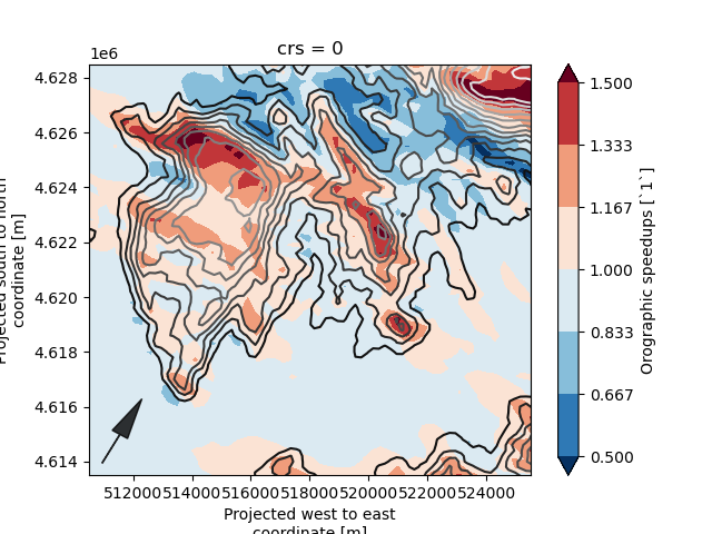
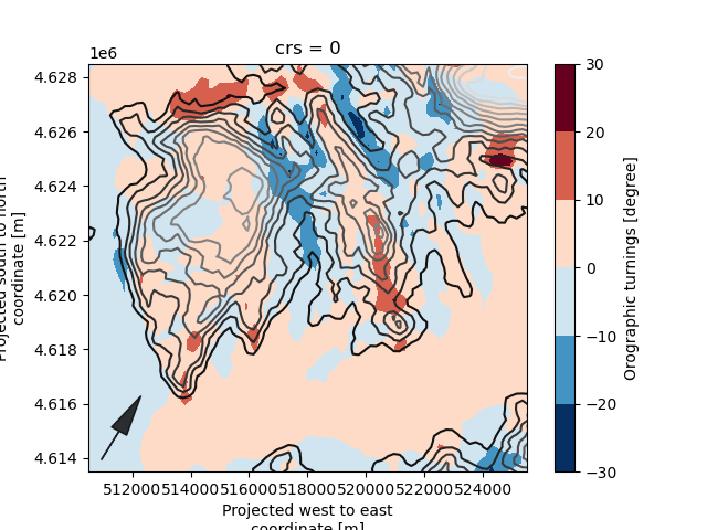
As expected, we see speed-ups on up-slope regions and slow-downs on down-slope regions. Next, we can take a look at the orographic turning:
In [33]: fig, ax = plt.subplots(1, 1)

In [34]: ax.set(xlim=(xmin, xmax), ylim=(ymin, ymax));

In [35]: (
   ....:     site_effects["orographic_turnings"]
   ....:     .sel(sector=210, height=50)
   ....:     .plot.contourf(center=0, ax=ax, add_colorbar=True)
   ....: );
   ....:

In [36]: plot_arrow(x=0.03, y=0.03, ws=0.08, wd=210, ax=ax);

In [37]: elev_raster.plot.contour(levels=16, cmap="gray", ax=ax, add_colorbar=False);
Now, let us plot the roughness speed-up:
In [38]: fig, ax = plt.subplots(1, 1)

In [39]: ax.set(xlim=(xmin, xmax), ylim=(ymin, ymax));

In [40]: (
   ....:     site_effects["roughness_speedups"]
   ....:     .sel(sector=210, height=50)
   ....:     .plot.contourf(vmin=0.8, vmax=1.2, cmap="RdBu_r", ax=ax, add_colorbar=True)
   ....: );
   ....:

In [41]: plot_arrow(x=0.03, y=0.03, ws=0.08, wd=210, ax=ax);

In [42]: z0_raster = pw.io.vector_to_raster(rgh_map, res=200)

In [43]: np.log1p(z0_raster).plot.contour(levels=16, cmap="gray", ax=ax, add_colorbar=False);
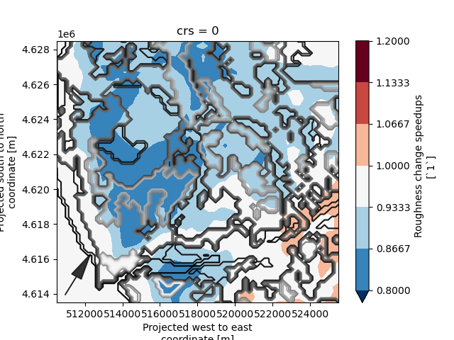
We can see large areas of slow-down of the flow as it transitions from low roughness over the sea to higher surface roughness over land. Remember, the roughness speed-ups shown here are the internal boundary layer effects, and not the geostrophic drag-law effects, which come in during the generalization and downscaling step, using the effective roughnesses stored in “z0meso”. It is also during these steps than any stability effects are accounted for.
Generalization#
The generalization step is the process of removing local terrain and surface layer effects from the observed wind climate and obtaining new idealized wind climates at a number of standard conditions (surface roughness and height above ground). We call this new wind climate a “Generalized Wind Climate” (GWC), because it is representative of a larger area than the observed wind climate. The fundamental assumption behind the method is that the geostrophic wind climate remains the same in a wider region around the original site, and that the observed wind climate is a perturbation of this geostrophic wind climate. The wind climate adjustments to the observed wind climate are done in this order: first the orographic and IBL speed-ups and turning are applied (inversely), then the geosteophic drag-law, including the stability correction is used to obtain the idealized wind climate(s).
To generalize a observed/binned wind climate, generalize() is used:
In [44]: gwc = pw.wasp.generalize(bwc, topo_map)

In [45]: print(gwc)
<xarray.Dataset> Size: 4kB
Dimensions:        (point: 1, sector: 12, gen_roughness: 5, gen_height: 5)
Coordinates:
    height         (point) float64 8B 25.3
    south_north    (point) float64 8B 4.621e+06
    west_east      (point) float64 8B 5.147e+05
  * sector         (sector) float64 96B 0.0 30.0 60.0 90.0 ... 270.0 300.0 330.0
    sector_ceil    (sector) float64 96B 15.0 45.0 75.0 ... 285.0 315.0 345.0
    sector_floor   (sector) float64 96B 345.0 15.0 45.0 ... 255.0 285.0 315.0
  * gen_roughness  (gen_roughness) float64 40B 0.0 0.03 0.1 0.4 1.5
  * gen_height     (gen_height) int64 40B 10 25 50 100 250
    crs            int8 1B 0
Dimensions without coordinates: point
Data variables:
    A              (sector, gen_height, gen_roughness, point) float32 1kB 5.6...
    k              (sector, gen_height, gen_roughness, point) float32 1kB 1.7...
    wdfreq         (sector, gen_height, gen_roughness, point) float32 1kB 0.0...
    site_elev      (point) float32 4B 381.0
Attributes:
    Conventions:      CF-1.8
    history:          2026-01-29T14:39:27+00:00:\twindkit==2.0.0\tcreate_data...
    description:      SerraSantaluzia
    Package name:     windkit
    Package version:  2.0.0
    Creation date:    2026-01-29T14:39:40+00:00
    Object type:      Geostrophic Wind Climate
    author:           Neil Davis
    author_email:     neda@dtu.dk
    institution:      DTU Wind and Energy Systems
    title:            Generalized wind climate
The result is a Generalized Wind Climate, which contains weibull parameters
for a number of surface roughnesses and heights
(prefixed with _gen to signify that these are conditions in the “generalization space”).
Note
The gen_heights and gen_roughnesses classes should be set to capture the characteristics at the site
as well as possible. It is recommended to select heights that cover all heights one wishes to predicted, and to include
specific heights of interest as standalone classes. The same goes for the surface roughness classes.
Note
pywasp.wasp.generalize() uses 1x runs in your PyWAsP subscription
Downscaling#
The downscaling step is the reverse process of the generalization step, where the generalized wind climate is used to obtain new wind climates at desired locations. The idealized wind climates from the GWC are interopolated to the actual characteristics of the desired output locations, using the local site effects and stability. Lastly, the orographic and IBL speed-ups and turning are applied to the wind climates to obtain the final wind climates at the desired locations.
To downscale a GWC to the desired output locations, using pre-calculated site_effects, downscale() is used:
In [46]: wwc = pw.wasp.downscale_from_site_effects(gwc, site_effects, interp_method="nearest")

In [47]: print(wwc)
<xarray.Dataset> Size: 386kB
Dimensions:       (height: 1, south_north: 51, west_east: 51, sector: 12)
Coordinates:
  * height        (height) int64 8B 50
  * south_north   (south_north) int64 408B 4613500 4613800 ... 4628200 4628500
  * west_east     (west_east) int64 408B 510500 510800 511100 ... 525200 525500
  * sector        (sector) float64 96B 0.0 30.0 60.0 90.0 ... 270.0 300.0 330.0
    sector_ceil   (sector) float64 96B 15.0 45.0 75.0 ... 285.0 315.0 345.0
    sector_floor  (sector) float64 96B 345.0 15.0 45.0 ... 255.0 285.0 315.0
    crs           int8 1B 0
Data variables:
    A             (sector, height, south_north, west_east) float32 125kB 6.60...
    k             (sector, height, south_north, west_east) float32 125kB 1.98...
    wdfreq        (sector, height, south_north, west_east) float32 125kB 0.06...
    site_elev     (south_north, west_east) float32 10kB 0.1 0.1 ... 773.6 781.0
Attributes:
    Conventions:      CF-1.8
    history:          2026-01-29T14:39:30+00:00:\twindkit==2.0.0\t"cuboid")\n...
    Package name:     windkit
    Package version:  2.0.0
    Creation date:    2026-01-29T14:39:40+00:00
    Object type:      Geostrophic Wind Climate
    author:           Neil Davis
    author_email:     neda@dtu.dk
    institution:      DTU Wind and Energy Systems
    title:            WAsP site effects
The predicted wind climate is a weibull wind climate, containing sector-wise weibull parameters for the desired locations.
To downscale without pre-calculating the site effects, pw.wasp.downscale()
can be used instead:
In [48]: wwc = pw.wasp.downscale(gwc, topo_map, output_locs, interp_method="nearest")
Note
pywasp.wasp.downscale() uses 1x runs in your PyWAsP subscription
One-step extrapolation#
For direct horizontal and vertical extrapolation of wind climates,
wherein the generalization and downscaling is done in a single call, the
predict_wwc() can be used.
In [49]: wwc = pw.wasp.predict_wwc(bwc, topo_map, output_locs)
The similar to doing the generalization and downscaling in two steps, the result is a weibull wind climate.
Another option is to use predict_bwc() to keep much of the structure of the empirical distribution and get a binned wind climate as output.
In [50]: bwc = pw.wasp.predict_bwc(bwc, topo_map, output_locs)

In [51]: print(bwc)
<xarray.Dataset> Size: 5MB
Dimensions:        (height: 1, south_north: 51, west_east: 51, sector: 12,
                    wsbin: 41)
Coordinates:
  * height         (height) int64 8B 50
  * south_north    (south_north) int64 408B 4613500 4613800 ... 4628200 4628500
  * west_east      (west_east) int64 408B 510500 510800 511100 ... 525200 525500
  * sector         (sector) float64 96B 0.0 30.0 60.0 90.0 ... 270.0 300.0 330.0
    sector_ceil    (sector) float64 96B 15.0 45.0 75.0 ... 285.0 315.0 345.0
    sector_floor   (sector) float64 96B 345.0 15.0 45.0 ... 255.0 285.0 315.0
  * wsbin          (wsbin) float64 328B 0.5 1.5 2.5 3.5 ... 37.5 38.5 39.5 40.5
    wsceil         (wsbin) float64 328B 1.0 2.0 3.0 4.0 ... 38.0 39.0 40.0 41.0
    wsfloor        (wsbin) float64 328B 0.0 1.0 2.0 3.0 ... 37.0 38.0 39.0 40.0
    crs            int8 1B 0
Data variables:
    wsfreq         (wsbin, sector, height, south_north, west_east) float32 5MB ...
    wdfreq         (sector, height, south_north, west_east) float32 125kB 0.0...
    site_elev      (south_north, west_east) float32 10kB 0.1 0.1 ... 773.6 781.0
    air_density    (height, south_north, west_east) float32 10kB 1.218 ... 1.126
    wspd           (height, south_north, west_east) float64 21kB 7.08 ... 7.918
    power_density  (height, south_north, west_east) float64 21kB 381.5 ... 475.3
Attributes:
    Conventions:      CF-1.8
    history:          2026-01-29T14:39:30+00:00:\twindkit==2.0.0\t"cuboid")\n...
    Package name:     windkit
    Package version:  2.0.0
    Creation date:    2026-01-29T14:40:10+00:00
    Object type:      Met fields
    author:           Neil Davis
    author_email:     neda@dtu.dk
    institution:      DTU Wind and Energy Systems
    title:            WAsP site effects
Note
pywasp.wasp.predict_wwc() and pywasp.wasp.predict_bwc() uses 2x runs in your PyWAsP subscription
WAsP Model Configuration#
When running WAsP through PyWAsP, there are a number of parameters that can be set through the
conf argument to the functions: TopographyMap.get_site_effects(),
generalize(), downscale_from_site_effects(), and downscale().
The conf input is a Config object contains the model parameters, and is set
by default to correspond to the WAsP GUI version 12.8, using the latest version of WAsP
and a set of pre-defined parameters for the terrain and climate models.
To use a previous version of WAsP or to fine tune the model parameters, we can create an instance
of the Config class, which then can be passed as an argument to the functions:
In [52]: conf = pw.wasp.Config("WAsP_12.7")  # Use a parameter-set from a previous WAsP version.

In [53]: wwc = pw.wasp.predict_wwc(
   ....:     bwc,
   ....:     topo_map,
   ....:     output_locs
   ....: )
   ....:
The Config object can be initialized with a str, as above, which uses
parameters from a specific version of WAsP:
“WAsP_11.4”: WAsP 11 profile model using c_g=1.65 and powerlaw estimation for reversal height. Classic terrain analysis.
“WAsP_12.6”: WAsP 12 profile model with c_g solved by iteration and dA/dmu set such that it corresponds with the old profile model. Classic terarin analysis
“WAsP_12.7”: WAsP 12 profile model, as version 12.6 but including baroclinicity. Spider terrain analysis.
“WAsP_12.8”: WAsP 12 profile model, including sectorwise stability and baroclinicity as described in mesoclimate class (Profile model 3); terrain analysis 1
See also
- WAsP Configuration Parameters
Complete reference of all terrain and climate model parameters with their default values and descriptions.
Initializing the object with no parameters, means the default, “WAsP_12.8”, is used. Once initialized, the object can also be further modified by manually chaging specific parameters.
The Config class sets parameters for the terrain and the climate WAsP models. An
instance of Config has two properties, climate and terrain, which are
instances of Climate and Terrain.
The detail of the set values can be check as follows:
config = pywasp.wasp.Config()
config.climate
"""
Index Parameter Current Default Description
value value
===== =============== ============ =========== ==================================================
10 a0 1.800000 1.8 A0 parameter in geostrophic drag law under neutral conditions
11 b0 4.500000 4.5 B0 parameter in neutral geostrophic drag law
56 rms_hfx_land 100.000000 100 Root mean square of heat flux over land
57 rms_hfx_water 30.000000 30 Rms Heatflux over water
58 off_hfx_land -40.000000 -40 Offset (mean) heatflux over land
59 off_hfx_water -8.000000 -8 Offset (mean) heatflux over water
60 stab_lim_land 1.000000 1 Factor on geostrophic height for stab envelope limiting
77 stab_lim_water 1.000000 1 Factor on geostrophic height (sea) for stability envelope limiting"""
config.terrain
"""
Index Parameter Current Default Description
value value
===== =============== ============ =========== ==================================================
31 decay_length 10000.000000 10000 Decay-length for importance of roughness relative to distance from center
67 max_no_rgh 10.000000 10 Max number of roughness changes per sector."""
The configuration values stored as key - value pairs and can be accessed or set individually by index
config.climate[10] = 3.6
config.climate
"""
Index  Parameter        Current       Default       Description
                        value         value
=====  ===============  ============  ===========   ==================================================
    10  a0                   3.600000  1.8           A0  parameter in geostrophic drag law under neutral conditions
    11  b0                   4.500000  4.5           B0 parameter in neutral geostrophic drag law
    56  rms_hfx_land       100.000000  100           Root mean square of heat flux over land
    57  rms_hfx_water       30.000000  30            Rms Heatflux over water
    58  off_hfx_land       -40.000000  -40           Offset (mean) heatflux over land
    59  off_hfx_water       -8.000000  -8            Offset (mean) heatflux over water
    60  stab_lim_land        1.000000  1             Factor on geostrophic height for stab envelope limiting
    77  stab_lim_water       1.000000  1             Factor on geostrophic height (sea) for stability envelope limiting"""
It is also possible to set a combination of values to define a climate profile model and a terrain analysis.
climate.set_profile_model(0)
terrain.set_terrain_analysis(1)
For further details of the above, check the API Reference Config.